Page 99 - Modern Control Systems

Section 2.5 The Transfer Function of Linear Systems 73
Disturbance

Armature Speed
T m(s) " T L(s)
K m I Position
W
R a + L as Js + b 0(.v)
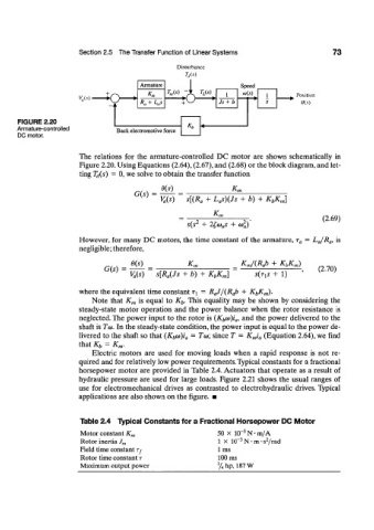
FIGURE 2.20
Armature-controlled Back electromotive force
DC motor.

The relations for the armature-controlled DC motor are shown schematically in
Figure 2.20. Using Equations (2.64), (2.67), and (2.68) or the block diagram, and let-
ting T d(s) = 0, we solve to obtain the transfer function
0(S) _ Kjn
G(s) =
V a(s) s[(R a + L as)(Js + b) + K bK m]

_ ^jn
(2.69)
s(s 2 + 2£<D ns + col)
However, for many DC motors, the time constant of the armature, r a = L a/R a, is
negligible; therefore,

e(s) K, K m/(R ab + KbK m)
G(s) = (2.70)
V a(s) s[R a(Js + b) + K bK m) S{T XS + 1)

where the equivalent time constant T\ = R aJ/{R ab + Kf,K m).
Note that K m is equal to K b. This equality may be shown by considering the
steady-state motor operation and the power balance when the rotor resistance is
neglected. The power input to the rotor is (K b(o)i a, and the power delivered to the
shaft is Tw. In the steady-state condition, the power input is equal to the power de-
livered to the shaft so that (K bco)i a = Tco; since T = K mi a (Equation 2.64), we find
that K b = K m.
Electric motors are used for moving loads when a rapid response is not re-
quired and for relatively low power requirements. Typical constants for a fractional
horsepower motor are provided in Table 2.4. Actuators that operate as a result of
hydraulic pressure are used for large loads. Figure 2.21 shows the usual ranges of
use for electromechanical drives as contrasted to electrohydraulic drives. Typical
applications are also shown on the figure. •

Table 2.4 Typical Constants for a Fractional Horsepower DC Motor
3
Motor constant K, n 50 X 10" N • m/A
3
2
Rotor inertia J m 1 X 10" N • m • s /rad
Field time constant Tf 1 ms
Rotor time constant T 100 ms
Maximum output power % hp, 187 W