Page 100 - Modern Control Systems

7 4 Chapter 2 Mathematical Models of Systems

500 i 1 1 1 1
400
300 . . _ .4 .. r Beyond present
Steel state of the art
200
mills
100
70
hydrostatic j
50
"
40 Cranes and
30 • hoists Range of
20 conventional
i .lectrohydraulk
10
control
7 1
t
5 Machine tools
4
3 Antennas
2 iRob JtS
Usus lly electromechanical
1 actuation 1 -
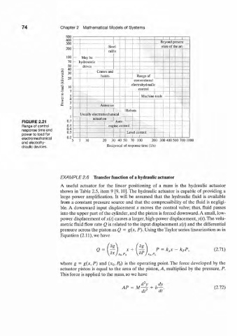
FIGURE 2.21 0.7 Auto
Range of control 0.5 --
response time and 0.4 . - [ '
0.3
power to load for
electromechanical 0.2 20 30 40 50 70 100 200 300 400 500 700 1000
and electrohy- 7 10
draulic devices. Reciprocal of response time (1/s)

EXAMPLE 2.6 Transfer function of a hydraulic actuator
A useful actuator for the linear positioning of a mass is the hydraulic actuator
shown in Table 2.5, item 9 [9,10]. The hydraulic actuator is capable of providing a
large power amplification. It will be assumed that the hydraulic fluid is available
from a constant pressure source and that the compressibility of the fluid is negligi-
ble. A downward input displacement x moves the control valve; thus, fluid passes
into the upper part of the cylinder, and the piston is forced downward. A small, low-
power displacement of x{t) causes a larger, high-power displacement,y(t). The volu-
metric fluid flow rate Q is related to the input displacement x(t) and the differential
pressure across the piston as Q = g(x, P). Using the Taylor series linearization as in
Equation (2.11), we have

Bg_
f x P = k xx - k FP, (2.71)
irl - dP v fb °H

where g = g(x, P) and (x 0, /¾) is the operating point. The force developed by the
actuator piston is equal to the area of the piston, A, multiplied by the pressure, P.
This force is applied to the mass, so we have
2
d y dy
AP = Af-4 + b-r. (2.72)
dt 2 dt