Page 84 - Modern Control Systems

58 Chapter 2 Mathematical Models of Systems

Mass M
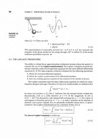
FIGURE 2.6
Pendulum
oscillator. (a) (b)
where 7^ = 0. Then, we have

T = MgL(cos O°)(0 - 0°)
= MgL6. (2.13)
This approximation is reasonably accurate for — ir/4 < Q < ir/4. For example, the
response of the linear model for the swing through ±30° is within 5% of the actual
nonlinear pendulum response. •

2.4 THE LAPLACE TRANSFORM

The ability to obtain linear approximations of physical systems allows the analyst to
consider the use of the Laplace transformation.The Laplace transform method sub-
stitutes relatively easily solved algebraic equations for the more difficult differential
equations [1,3].The time-response solution is obtained by the following operations:
1. Obtain the linearized differential equations.
2. Obtain the Laplace transformation of the differential equations.
3. Solve the resulting algebraic equation for the transform of the variable of interest.
The Laplace transform exists for linear differential equations for which the trans-
formation integral converges.Therefore, for f(t) to be transformable, it is sufficient that

I \f{t)\e**tu < oo,

for some real, positive o- 5 [1]. The 0~ indicates that the integral should include any
discontinuity, such as a delta function at t — 0. If the magnitude of f(t) is
al
\f(t) | < Me for all positive t, the integral will converge for a^ > a. The region of
convergence is therefore given by oo > <r ( > a, and crj is known as the abscissa of
absolute convergence. Signals that are physically realizable always have a Laplace
transform. The Laplace transformation for a function of time,/(i), is

(2.14)

The inverse Laplace transform is written as

(2.15)