Page 82 - Modern Control Systems

56 Chapter 2 Mathematical Models of Systems

second system may be considered linear about an operating point JC 0 , )¾ for small
changes Ax and Ay. When x = XQ + Ax and y = y 0 + Ay, we have

y = mx + b
or
+ Ay = + m Ax + b.
y 0 mx 0
Therefore, Ay = m Ax, which satisfies the necessary conditions.
The linearity of many mechanical and electrical elements can be assumed over a
reasonably large range of the variables [7]. This is not usually the case for thermal and
fluid elements, which are more frequently nonlinear in character. Fortunately, how-
ever, one can often linearize nonlinear elements assuming small-signal conditions. This
is the normal approach used to obtain a linear equivalent circuit for electronic circuits
and transistors. Consider a general element with an excitation (through-) variable x(t)
and a response (across-) variable y(t). Several examples of dynamic system variables
are given in Table 2.1. The relationship of the two variables is written as

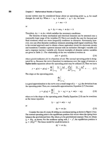
y(t) = g(*(0). (2.6)
where g(x(t)) indicates y(t) is a function of x(t).The normal operating point is desig-
nated by x 0. Because the curve (function) is continuous over the range of interest, a
Taylor series expansion about the operating point may be utilized [7]. Then we have

dg (* - XQ) d g (x - x 0) 2
2
y = g(x) = g(x 0) + — 1! dx 2 „ + •••• (2.7)
x=x 0
The slope at the operating point,

dx
is a good approximation to the curve over a small range of (x - x 0), the deviation from
the operating point. Then, as a reasonable approximation, Equation (2.7) becomes

y = g(*o) + - - (x - x 0) = y 0 + m(x - x Q), (2.8)
x=x 0
where m is the slope at the operating point. Finally, Equation (2.8) can be rewritten
as the linear equation
(y - y 0) = m(x - x 0)
or
Ay = m Ax. (2.9)
Consider the case of a mass,M, sitting on a nonlinear spring, as shown in Figure 2.5(a).
The normal operating point is the equilibrium position that occurs when the spring force
balances the gravitational force Mg, where g is the gravitational constant. Thus, we obtain
2
= Mg, as shown. For the nonlinear spring with / = y , the equilibrium position is
/ 0 1 2
y 0 = (Mg) / . The linear model for small deviation is
A/ = m Ay,