Page 203 - Modern Control of DC-Based Power Systems

Control Approaches for Parallel Source Converter Systems 167

with the buck converter system including the LC-output filter which
corresponds to a second-order system.

ðÞUx 2
_ x 1 5 f 1 x 1 1 h 1 x 1
(5.148)
ðÞ
_ x 2 5 u
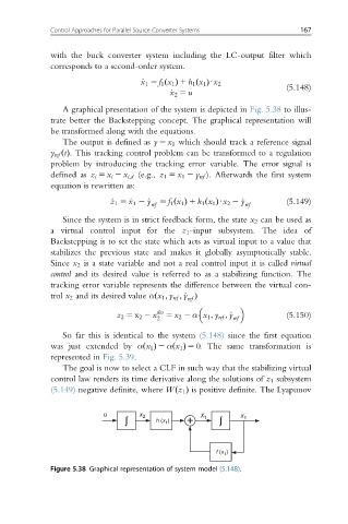
A graphical presentation of the system is depicted in Fig. 5.38 to illus-
trate better the Backstepping concept. The graphical representation will
be transformed along with the equations.
The output is defined as y 5 x 1 which should track a reference signal
y ref ðtÞ. This tracking control problem can be transformed to a regulation
problem by introducing the tracking error variable. The error signal is
defined as z i 5 x i 2 x i;d (e.g., z 1 5 x 1 2 y ref ). Afterwards the first system
equation is rewritten as:

ðÞUx 2 2 _y (5.149)
_ z 1 5 _x 1 2 _y 5 f 1 x 1 1 h 1 x 1
ref ðÞ ref
Since the system is in strict feedback form, the state x 2 can be used as
a virtual control input for the z 1 -input subsystem. The idea of
Backstepping is to set the state which acts as virtual input to a value that
stabilizes the previous state and makes it globally asymptotically stable.
Since x 2 is a state variable and not a real control input it is called virtual
control and its desired value is referred to as a stabilizing function. The
tracking error variable represents the difference between the virtual con-
ref
trol x 2 and its desired value αðx 1 ; y ref ; _y Þ

des
z 2 5 x 2 2 x 5 x 2 2 α x 1 ; y ref ; _y (5.150)
2 ref
So far this is identical to the system (5.148) since the first equation
was just extended by α x 1 2 α x 1 5 0. The same transformation is
ðÞ
ðÞ
represented in Fig. 5.39.
The goal is now to select a CLF in such way that the stabilizing virtual
control law renders its time derivative along the solutions of z 1 subsystem
(5.149) negative definite, where Wz 1 is positive definite. The Lyapunov
ðÞ

u x 2 Ẋ x
ʃ h (x ) + 1 ʃ 1
1

f (x )
1
Figure 5.38 Graphical representation of system model (5.148).