Page 204 - Modern Control of DC-Based Power Systems

168 Modern Control of DC-Based Power Systems

u x 2 Ẋ Ẋ x 1
ʃ + h (x ) + 1 1 ʃ
1
–
α (x )
1
f (x ) + h (x )α (x )
1
1
1
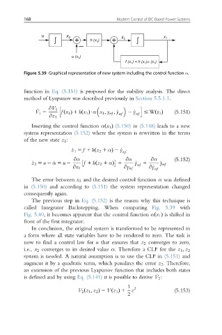
Figure 5.39 Graphical representation of new system including the control function α.

function in Eq. (5.151) is proposed for the stability analysis. The direct
method of Lyapunov was described previously in Section 5.5.1.1.

h i
@V 1
_ V 1 5 fx 1 1 hx 1 ref 2 _y ref # Wz 1 (5.151)
ðÞUα x 1 ; y ref ; _y
ðÞ
ðÞ
@z 1
Inserting the control function α x 1 (5.150) in (5.148) leads to a new
ðÞ
system representation (5.152) where the system is rewritten in the terms
of the new state z 2 :
Þ 2 _y
_ z 1 5 f 1 hz 2 1 αð ref
@α @α (5.152)

_ z 2 5 u 2 _ α 5 u 2 @α f 1 hz 2 1 αÞ 1 _ y 1
ref ÿ ref
ð
@x 1 @y ref @_y
ref
The error between x 2 and the desired control function α was defined
in (5.150) and according to (5.151) the system representation changed
consequently again.
The previous step in Eq. (5.152) is the reason why this technique is
called Integrator Backstepping. When comparing Fig. 5.39 with
Fig. 5.40, it becomes apparent that the control function α x 1 is shifted in
ðÞ
front of the first integrator.
In conclusion, the original system is transformed to be represented in
a form where all state variables have to be rendered to zero. The task is
now to find a control law for u that ensures that z 2 converges to zero,
i.e., x 2 converges to its desired value α. Therefore a CLF for the z 1 ; z 2
system is needed. A natural assumption is to use the CLF in (5.151) and
augment it by a quadratic term, which penalizes the error z 2 . Therefore,
an extension of the previous Lyapunov function that includes both states
is defined and by using Eq. (5.141) it is possible to derive _ V 2 :

1 2
V 2 z 1 ; z 2 Þ 5 Vz 1 1 z (5.153)
ð
ðÞ
2