Page 113 - Modern Optical Engineering The Design of Optical Systems

96 Chapter Five

Note that in an H′–tan U′ plot, this plotting convention violates the
convention for the sign of the ray slope. This seeming contradiction is
the result of the change from the historical optical ray slope sign
convention which occurred several decades ago.
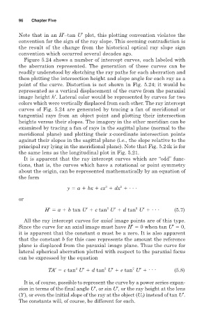
Figure 5.24 shows a number of intercept curves, each labeled with
the aberration represented. The generation of these curves can be
readily understood by sketching the ray paths for each aberration and
then plotting the intersection height and slope angle for each ray as a
point of the curve. Distortion is not shown in Fig. 5.24; it would be
represented as a vertical displacement of the curve from the paraxial
image height h′. Lateral color would be represented by curves for two
colors which were vertically displaced from each other. The ray intercept
curves of Fig. 5.24 are generated by tracing a fan of meridional or
tangential rays from an object point and plotting their intersection
heights versus their slopes. The imagery in the other meridian can be
examined by tracing a fan of rays in the sagittal plane (normal to the
meridional plane) and plotting their x-coordinate intersection points
against their slopes in the sagittal plane (i.e., the slope relative to the
principal ray lying in the meridional plane). Note that Fig. 5.24k is for
the same lens as the longitudinal plot in Fig. 5.21.
It is apparent that the ray intercept curves which are “odd” func-
tions, that is, the curves which have a rotational or point symmetry
about the origin, can be represented mathematically by an equation of
the form
5
3
y a bx cx dx . . .
or
3
5
H′ a b tan U′ c tan U′ d tan U′ . . . (5.7)
All the ray intercept curves for axial image points are of this type.
Since the curve for an axial image must have H′ 0 when tan U′ 0,
it is apparent that the constant a must be a zero. It is also apparent
that the constant b for this case represents the amount the reference
plane is displaced from the paraxial image plane. Thus the curve for
lateral spherical aberration plotted with respect to the paraxial focus
can be expressed by the equation

5
7
3
TA′ c tan U′ d tan U′ e tan U′ . . . (5.8)
It is, of course, possible to represent the curve by a power series expan-
sion in terms of the final angle U′, or sin U′, or the ray height at the lens
(Y), or even the initial slope of the ray at the object (U 0 ) instead of tan U′.
The constants will, of course, be different for each.