Page 133 - Modern Spatiotemporal Geostatistics

114 Modern Spatiotemporal Geostatistics — Chapter 5

etc. As before, the BME analysis can easily be extended to include all the
mapping points t mop.

COMMENT 5.5: W e can proceed further with the mathematical formulations

above i n a number o f ways. Consider, e.g., Equations5.20 an d 5.21 a t a

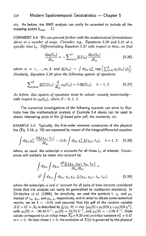
specific time t a .Differentiating Equation 5. 21 with respect to time, we find

where

Similarly, Equation 5.20 gives the following system of equations

As before, this system of equations must be solved—usually numerically —

with respect t o fJ-p(t a), where /3 = 0 , 1 , 2.

The numerical investigations of the following example can serve to illus-
trate how the mathematical analysis of Example 5.4 above can be used to
obtain interesting plots of the ^-based prior pdf, the moments, etc.
EXAMPLE 5.5: Typically, the first-order moment constraints of the physical
law (Eq. 3.16, p. 79) are expressed by means of the integrodifferential equation

where, as usual, the subscript a accounts for all times t a of interest. Covari-
ances will similarly be taken into account by

where the subscripts a and a' account for all pairs of time instants considered
(note that the analysis can easily be generalized to multipoint statistics). In
Christakos et al. (1999), for simplicity, we used the symbols t, \, and /UA
instead of t a, \a, and ^ a,\, respectively, and in order to obtain some numerical
results, we let b = -0.01 and assumed that the pdf of the random variable
2
X(t = Q) = X 0 is described by / ff( X; 0) = exp [Mo(0)+/ii(0)&x+ju 2(0)6x ],
with /z0(0) = -90.40 b'1, ^i(O) = JL9.54 b~l, and /x2(0) = -1.06 b'1; these
values correspond to an initial mean Xo = 9.20 and an initial variance d§ = 0.47
at t = 0. At later times t > 0, the evolution of X(t) is governed by the physical