Page 136 - Modern Spatiotemporal Geostatistics

Mathematical Formulation of the BME Method 117

We continue our discussion with a situation in which the coefficient of
the differential equation representing the physical law is a spatial random field
(i.e., a function of space). This situation possesses some interesting features
that can also be taken into consideration by the BME analysis.
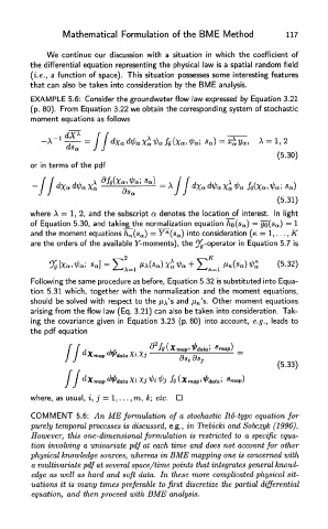
EXAMPLE 5.6: Consider the groundwater flow law expressed by Equation 3.21
(p. 80). From Equation 3.22 we obtain the corresponding system of stochastic
moment equations as follows

or in terms of the pdf

where A = 1, 2, and the subscript a denotes the location_pf interest. In light
of Equation 5.30, and taking the normalization equatio
K
and the moment equations h K(s a) = Y (s a) into consideration (K = I,... ,K
are the orders of the available F-moments), the 9^-operator in Equation 5.7 is

Following the same procedure as before, Equation 5.32 is substituted into Equa-
tion 5.31 which, together with the normalization and the moment equations,
should be solved with respect to the n\'s and fj, K's. Other moment equations
arising from the flow law (Eq. 3.21) can also be taken into consideration. Tak-
ing the covariance given in Equation 3.23 (p. 80) into account, e.g., leads to
the pdf equation

where, as usual, i, j = 1,..., m, k; etc.

COMMENT 5.6 : An M E formulation of a stochastic Ito-type equation fo r

purely temporal processes is discussed, e.g., in Trebicki an d Sobczyk (1996).

However, this one-dimensional formulation is restricted to a specific equa-
tion involving a univariate pdf at each time and does not account for other
physical knowledge sources, whereas in BME mapping one is concerned with

a multivariate pdf at several space/time points that integrates general knowl-
edge as well as hard and soft data. In these more complicated physical sit-

uations it is many times preferable to first discretize the partial differential

equation, and then proceed with BME analysis.