Page 134 - Modern Spatiotemporal Geostatistics

Mathematical Formulation of the BME Method 1 1 5

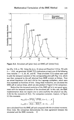
Figure 5.2. Simulated pdf (plain line) and BME pdf (dotted line).

law (Eq. 3.16, p. 79). Using the f g (%; 0) above and Equation 3.16 (p. 79) with
b = -0.01, we generated 10,000 -X"(£)-realizations at each one of the following
time instants: t = 0, 20, 40, and 60. These simulated X(£)-values were used
to plot the temporal evolution of the corresponding prior pdf (Fig. 5.2), which
was then compared to the pdf obtained from BME analysis as follows. First
we solved Equations 5.28 and 5.29 for the Lagrange multipliers, which were
thus expressed as functions of time. Using these multipliers, we calculated the
BME pdf at various times, which are also plotted in Figure 5.2 for comparison.
Notice that the temporal evolution of the BME pdf is in very good agree-
ment with the temporal evolution of the simulated pdf. In this case, the BME
implementation does not require one to solve explicitly the physical law (Eq.
3.16) for the moments of X(t). For comparison purposes, however, in Figure
5.3 the moments

were calculated from the BME pdf and compared with the simulated moments.
Once more, the comparison demonstrates the close agreement between the
simulated and the BME moments.