Page 207 - Modern Spatiotemporal Geostatistics

188 Modern Spatiotemporal Geostatistics — Chapter 9

we were to assume that there are no confounding factors. In Example 9.15,
below, the incorporation of a confounder into PEP analysis is demonstrated by
using particulate matter (PMio) data.

EXAMPLE 9.14: Temperature-mortality relationships are known to be V--
shaped, with both cold and hot temperature extremes resulting in higher death
rates (Saez et al, 1995; Christophersen, 1997). However, the North Carolina
region did not experience any substantial hot temperature extremes for the
time period considered (season 5, which corresponds—roughly—to the winter
of 1996); the daily mean temperature during season 5 did not exceed 65° F,
which is less than the 91° F threshold suggested by Honda et al. (1995) for
mortality increase induced by high temperature. Therefore, only low tempera-
tures were considered as the environmental exposure that could lead to higher
death rates.
The temperature field T(s, t) is a physical variable that is measured in
degrees Fahrenheit (° F) at the weather stations. These temperature mea-
surements are considered as hard data (i.e., there is a high degree of confi-
dence that the data obtained are not contaminated by errors). For the pur-
poses of human-exposure analysis, we defined the exposure to temperature
field X(s, t) = -K x T(s, t), where K = 4.4729 x ICT 2 is a constant cho-
sen such that the measured temperature exposure X-values have the same
stochastic mean as the measured death rates D; the negative sign ensures a
positive correlation between D and X (which, in this case, is considered as the
temperature exposure). Clearly, as the temperature T drops, the exposure to
cold temperature X increases and the death rate D is expected to increase.
The information available for mortality D(s, t) consists of daily death counts
for 14 representative counties and their aggregated neighbors. Death counts
provide an uncertain information about the death rate that can be expressed in
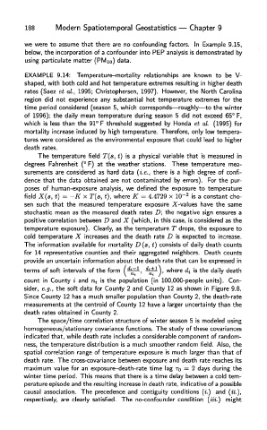
terms of soft intervals of the form wheredi is the daily death
count in County i and n» is the population (in 100,000-people units). Con-
sider, e.g., the soft data for County 2 and County 12 as shown in Figure 9.8.
Since County 12 has a much smaller population than County 2, the death-rate
measurements at the centroid of County 12 have a larger uncertainty than the
death rates obtained in County 2.
The space/time correlation structure of winter season 5 is modeled using
homogeneous/stationary covariance functions. The study of these covariances
indicated that, while death rate includes a considerable component of random-
ness, the temperature distribution is a much smoother random field. Also, the
spatial correlation range of temperature exposure is much larger than that of
death rate. The cross-covariance between exposure and death rate reaches its
maximum value for an exposure-death-rate time lag TO = 2 days during the
winter time period. This means that there is a time delay between a cold tem-
perature episode and the resulting increase in death rate, indicative of a possible
causal association. The precedence and contiguity conditions (i.) and (ii.),
respectively, are clearly satisfied. The no-confounder condition (m.) might