Page 233 - Modern Spatiotemporal Geostatistics
P. 233
214      Modern Spatiotemporal Geostatistics —   Chapter  10

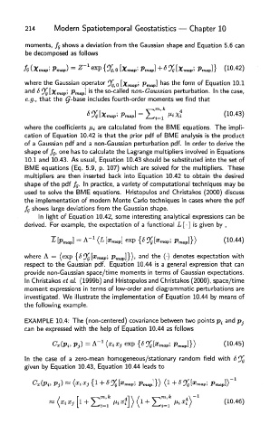
        moments,  f g  shows a deviation  from  the  Gaussian shape and Equation  5.6 can
        be decomposed as follows


        where the  Gaussian operator  9£,o [xmapj PmaP] nas the form of Equation 10.1
        and S 9£ [Xmap> Pmap] 's tne so-called non-Gaussian perturbation. In the case,
        e.g.,  that the  £-base includes fourth-order  moments we find that


        where the  coefficients  /z$  are calculated from  the  BME  equations.  The  impli-
        cation  of  Equation  10.42  is that  the  prior  pdf  of  BME  analysis  is the  product
        of  a Gaussian  pdf  and a non-Gaussian  perturbation  pdf.  In order to  derive  the
        shape of f g, one has to calculate the  Lagrange multipliers  involved in Equations
        10.1  and  10.43.  As usual,  Equation  10.43  should be substituted into the  set of
        BME  equations (Eq.  5.9,  p.  107)  which  are solved for  the  multipliers.  These
        multipliers  are then  inserted  back  into  Equation  10.42  to  obtain  the  desired
        shape of  the  pdf  fg.  In  practice,  a variety of computational  techniques may be
        used  to  solve the  BME  equations.  Hristopulos  and  Christakos (2000)  discuss
        the  implementation  of  modern  Monte  Carlo techniques in  cases where the  pdf
        fg  shows large deviations from  the  Gaussian  shape.
            In  light  of  Equation  10.42,  some  interesting  analytical expressions can be
        derived.  For example, the  expectation  of  a functional  L [ - ]  is given  by ,


        where                             anc' tne (') denotes expectation with
        respect  to  the  Gaussian  pdf.  Equation  10.44  is a general expression  that  can
        provide  non-Gaussian space/time  moments in terms of  Gaussian expectations.
        In Christakos et al.  (1999b) and Hristopulos and Christakos (2000),  space/time
        moment  expressions  in terms of  low-order  and diagrammatic perturbations are
        investigated.  We  illustrate  the  implementation  of  Equation  10.44  by means  of
        the  following example.

        EXAMPLE   10.4:  The  (non-centered)  covariance  between two  points p i  and p,j
        can  be expressed with the  help of  Equation  10.44  as follows


        In  the  case  of  a  zero-mean  homogeneous/stationary  random  field  with  <59£
        given  by Equation  10.43,  Equation  10.44  leads  to

