Page 234 - Modern Spatiotemporal Geostatistics

Single-Point Analytical Formulations 215

After some algebraic manipulations involving the properties of Gaussian expec-
tations, Equation 10.46 yields

2
where a% = (x ) and the p, is calculated from the BME equations. Equation
10.47 offers a good approximation in the case of a small deviation of the pdf
fg from the Gaussian shape (i.e., the non-Gaussian perturbation is sufficiently
weak). Similarly, the fourth-order moment is given by

Higher order moments are derived in a similar manner.

Approximate but in many cases useful analytical expressions are obtained
in terms of perturbation expansions. In the following example we compare two
analytical approximations and a numerical method.

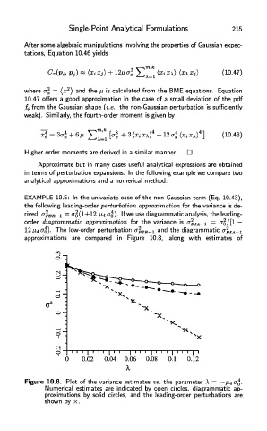
EXAMPLE 10.5: In the univariate case of the non-Gaussian term (Eq. 10.43),
the following leading-order perturbation approximation for the variance is de-
2
rived, cr , BB_ 1 = 0-0(1+12 /i4 CTO). If we use diagrammatic analysis, the leading-
order diagrammatic approximation for the variance is
2
12/^40-0]. The low-order perturbation <T , Bfi_ 1 and the diagrammatic
approximations are compared in Figure 10.8, along with estimates of

Figure 10.8. Plot of the variance estimates vs. the parameter
Numerical estimates are indicated by open circles, diagrammatic ap-
proximations by solid circles, and the leading-order perturbations are
shown by x.