Page 253 - Modern Spatiotemporal Geostatistics

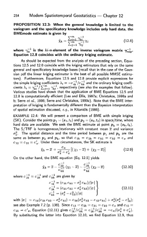
234 Modern Spatiotemporal Geostatistics — Chapter 12

PROPOSITION 12.3: When the general knowledge is limited to the
variogram and the specificatory knowledge includes only hard data, the
BMEmode estimate is given by

where j ki is the fcz-th element of the inverse variogram matrix
Equation 12.8 coincides with the ordinary kriging estimate.
As should be expected from the analysis of the preceding section, Equa-
tions 12.5 and 12.8 coincide with the kriging estimators that rely on the same
general and specificatory knowledge bases (recall that in the case of the Gaus-
sian pdf the linear kriging estimator is the best of all possible MMSE estima-
tors). Furthermore, Equations 12.5 and 12.8 provide explicit expressions
the simple kriging coefficient and the ordinary kriging coeffi-
cients respectively (see also the examples that follow).
Various studies have shown that the application of BME Equations 12.5 and
12.8 is computationally efficient (Lee and Ellis, 1997a; Christakos, 1998a and
b; Serre et al, 1998; Serre and Christakos, 1999a). Note that the BME inter-
pretation of kriging is fundamentally different than the Bayesian interpretation
of spatial estimation discussed, e.g., in Kitanidis (1986).
EXAMPLE 12.4: We will present a comparison of BME with simple kriging
(SK). Consider the points p l = (si,ti) andp 2 = (*2,*2) in space/time, where
hard data are available. We seek the BME estimate at point p k = (sfc,ifc).
The S/TRF is homogeneous/stationary with constant mean ~x and variance
a%- The spatial distance and the time period between p l and p k are the
same as between p 2 and p k, so that c\k = c-ik = Cki — cut = c x and
d2 = c 2i = c'. Under these circumstances, the SK estimate is

On the other hand, the BME equation (Eq. 12.5) yields

where and are given by

with
see also Example 7.2 (p. 138). Since i and
Equation (12.11) gives
By substituting the latter into Equation 12.10, we find Equation 12.9, thus