Page 255 - Modern Spatiotemporal Geostatistics

236 Modern Spatiotemporal Geostatistics — Chapter 12

To make some numerical comparisons between BME and kriging, a sim-
ulation study is examined below. The fact that BME can account for both
hard and soft data allows it to produce more accurate numerical results than
SK, which relies only on hard data. Remarkably, this is true even when SK is
allowed to use all hard data available, while BME is restricted to using only a
few hard data points.
EXAMPLE 12.6: Let us revisit Example 8.2 (p. 151). The estimates XaLsiPk)
obtained by BME at locations p k e D, which are the nodes of a dense grid
covering the shaded region D in Figure 8.1, can be compared with the es-
timates Xsi((Pk) obtained by space/time SK. For each realization x^(Pk)
(t = 1, 2, ..., 200), the estimation errors
were computed at all p k e D for both / = BME and SK. The difference
was calculated for each realization, and
the average over all 200 realizations was obtained at each point p k e D by
where the averaging operator
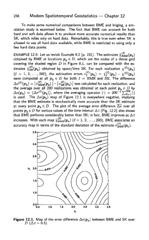
is used. The Ae(p fc) map of Figure 12.1 is everywhere negative, implying
that the BME estimate is stochastically more accurate than the SK estimate
at every point p k € D. The plot of the average error difference Ae over all
points Pk&D for various values of the time interval At (Fig. 12.2) also shows
that BME performs considerably better than SK; in fact, BME improves as At
2
increases. With each map XBMis(Pk) (t — 1> > • • • > 200), BME associates an
accuracy map in terms of the standard deviation of the estimate f

Figure 12.1. Map of the error difference Ae(p fe) between BME and SK over
D (At = 0.5).