Page 259 - Modern Spatiotemporal Geostatistics

240 Modern Spatiotemporal Geostatistics — Chapter 12

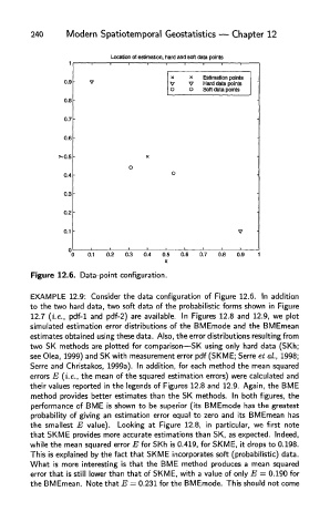
Figure 12.6. Data-point configuration.

EXAMPLE 12.9: Consider the data configuration of Figure 12.6. In addition
to the two hard data, two soft data of the probabilistic forms shown in Figure
12.7 (i.e., pdf-1 and pdf-2) are available. In Figures 12.8 and 12.9, we plot
simulated estimation error distributions of the BMEmode and the BMEmean
estimates obtained using these data. Also, the error distributions resulting from
two SK methods are plotted for comparison—SK using only hard data (SKh;
see Olea, 1999) and SK with measurement error pdf (SKME; Serre et al, 1998
Serre and Christakos, 1999a). In addition, for each method the mean squared
errors E (i.e., the mean of the squared estimation errors) were calculated and
their values reported in the legends of Figures 12.8 and 12.9. Again, the BME
method provides better estimates than the SK methods. In both figures, the
performance of BME is shown to be superior (its BMEmode has the greatest
probability of giving an estimation error equal to zero and its BMEmean has
the smallest E value). Looking at Figure 12.8, in particular, we first note
that SKME provides more accurate estimations than SK, as expected. Indeed,
while the mean squared error E for SKh is 0.419, for SKME, it drops to 0.198.
This is explained by the fact that SKME incorporates soft (probabilistic) data.
What is more interesting is that the BME method produces a mean squared
error that is still lower than that of SKME, with a value of only E = 0.190 for
the BMEmean. Note that E = 0.231 for the BMEmode. This should not come