
Page 254 - Modern Spatiotemporal Geostatistics
P. 254
Popular Methods in the Light of Modern Geostatistics 235
showing that the BME and SK estimates coincide in this case (which is an
expected result).
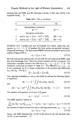
Table 12.1. The g a functions.
Normalization constraint
Variogram constraints
EXAMPLE 12.5: Consider the case of Example 12.4 above, where the vari-
ograms 7^ (i, j = 1, 2, k) between the three points are spatially isotropic/
temporally stationary. The well-known MMSE estimate provided by space/time
ordinary kriging (OK) is
We will compare the estimate (Eq. 12.12) with the one obtained by BME using
the same knowledge base. Since the known statistics are the variograms, the
information available concerns the differences The
statistical constraints are shown in Table 12.1. The difference
is not considered, for it is a linear combination of the previous two differences
d lk and V2fe- The OC
The Lagrange multipliers //i and (12 are found by solving the following system
of equations
and
The solution of Equations 12.14 and 12.15 gives
The BME equation reduces to
the solution of which is (note that due to isotropy/stationarity,
Hence, the BME estimate (Eq. 12.18) is the same as the OK estimate (Eq.
12.12), as was expected.