Page 264 - Modern Spatiotemporal Geostatistics

Popular Methods in the Light of Modern Geostatistics 245

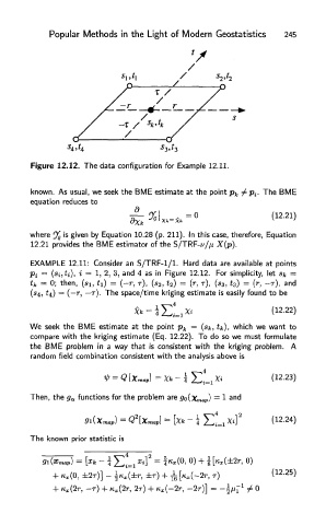
Figure 12.12. The data configuration for Example 12.11.

known. As usual, we seek the BME estimate at the point p k ^ p^ The BME
equation reduces to

s
where 9$ ' given by Equation 10.28 (p. 211). In this case, therefore, Equation
12.21 provides the BME estimator of the S/JRf-v/fi X(p).
EXAMPLE 12.11: Consider an S/TRF-1/1. Hard data are available at points
Pi = (si,ti), i = 1, 2, 3, and 4 as in Figure 12.12. For simplicity, let Sk =
t k = 0; then, (si, ti) = (-r, T), (s 2) * 2) = (r, r), (s 3, * 3) = (r, -T), and
(54, £4) = (—r, -T). The space/time kriging estimate is easily found to be

We seek the BME estimate at the point p k = (sk, tk), which we want to
compare with the kriging estimate (Eq. 12.22). To do so we must formulate
the BME problem in a way that is consistent with the kriging problem. A
random field combination consistent with the analysis above is

Then, the g a functions for the problem are <7 and

The known prior statistic is