Page 265 - Modern Spatiotemporal Geostatistics

246 Modern Spatiotemporal Geostatistics — Chapter 12

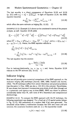
The last equality is a direct consequence of Equations 10.28 and 10.29
(p. 211) with CQ = &1 = gi&mp). In light of Equation 12.24, the BME
equation becomes

which offers the same estimate as kriging (Eq. 12.22).

EXAMPLE 12.12: Example 12.5 above can be considered in terms of the present
analysis, as well. Equation 10.28 yields

wherwe and
Hence, the BME equation reduces to

The last equation has the solution

Due to isotropy/stationarity, jik = 72*; = 7 and, hence, Equation 12.29
reduces to the OK estimate (Eq. 12.12).

Indicator kriging

Next we will provide some numerical comparisons of the BME approach vs. the
indicator kriging (IK) technique (Journel, 1986, 1989; Deutsch and Journel,
1992). The IK technique suffers from certain theoretical and practical problems
(see discussion in Olea, 1999; see also p. 133-34 in this volume). Nevertheless,
IK was chosen here because it incorporates some kinds of soft data (though not
in a systematic and rigorous way as does BME). BME was shown to perform
considerably better than IK, with none of IK's theoretical and computational
shortcomings.
EXAMPLE 12.13: To compare the BME approach with the IK technique, the
following experiment was designed. For a fixed set of 13 spatial points (shown
in Fig. 12.13), 500 realizations of a random field X(p) were generated. The
simulated values follow a multivariate Gaussian law with zero mean and unit
variance; the covariance functions used are: (i.) the exponential model