Page 53 - Modern Spatiotemporal Geostatistics

34 Modern Spatiotemporal Geostatistics — Chapter 2

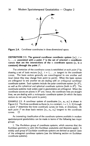
Figure 2.4. Curvilinear coordinates in three-dimensional space.

DEFINITION 2.1: The general curvilinear coordinate system {s ; }, i =
1,... ,n associated with a point P is the set of oriented n coordinate
curves that are the intersections of the n coordinate spaces (s, is a
constant) through the point P.
The orientation of the coordinate curves is established at each point P by
drawing a set of basis vectors {ei} , i = 1,... , n tangent to the coordinate
curves. The basis vectors generally are nonorthogonal to one another and
local (since they may change from point to point). When the basis vectors
are orthogonal to one another we are dealing with an orthogonal curvilinear
2
coordinate system. Such systems include the polar coordinate system (in R ),
3
as well as the cylindrical and spherical coordinate systems (both in R ). The
coordinate systems most widely used in geostatistics are orthogonal. When the
coordinate spaces are planes in R 3 and, hence, the coordinate lines are straight
lines, we are dealing with a rectangular coordinate system (in which the basis
vectors do not vary from point to point).

EXAMPLE 2.5: A curvilinear system of coordinates {si, 82, 83} is shown in
Figure 2.4. The three coordinate surfaces (s, is a constant, i = 1,2, 3) through
a point P determine the three coordinate curves (or lines, or directions). At
each point P we draw basis vectors {e\, e%, 63} tangent to the coordinate
curves.
An interesting classification of the coordinate systems available in modern
spatiotemporal geostatistics can be made in terms of the following two major
groups:
1. The Euclidean group of coordinate systems, which assumes that the
Euclidean geometry is valid (the Euclidean postulates and theorems apply). A
widely used group of Euclidean coordinate systems are derived as special cases
of the orthogonal curvilinear systems (see the following section on Euclidean
coordinate systems).