Page 297 - Book Hosokawa Nanoparticle Technology Handbook

FUNDAMENTALS CH. 5 CHARACTERIZATION METHODS FOR NANOSTRUCTURE OF MATERIALS
The recent studies on the above theoretical peak profile ambiguous, if sufficient size broadening is observed
have elucidated that the theoretical profile becomes and the experimental line profile can be approximated
close to the Lorentzian shape in the case where about by the Lorentzian peak shape. In such a case, log-
70% of the whole crystallites have the size within the normally distributed size and spherical shape of the
range from half to twice of the median size, and crystallites can be assumed as described above. The
“super-Lorentzian” shape with sharpened peak-top dependence of the Lorentzian width on the diffraction
and long tails is predicted for broader distribution of angle is appropriately modeled by equation (5.2).
the crystallite size [2]. Figs. 5.2.1 and 5.2.2 show the Since the two parameters and can be treated as
X
Y
probability density function of the log-normal distri- adjustable parameters in the Rietveld method to fit the
bution function and the corresponding theoretical experimental data, the optimized values are automati-
peak profiles. cally estimated by iterative calculations. The analyti-
Although the Rietveld method [11] is mainly aimed cal method assuming the Voigtian profile, which is
to refine the crystal structure from the powder dif- defined by the convolution of the Lorentzian and
fraction data, it can also be applied to the evaluation Gaussian (normal distribution) functions, has also
of crystallite size. The application of the Rietveld been proposed [12].
method to evaluate the crystallite size will be less

References
2.0 [1] W.A. Rachinger: J. Sci. Instrum., 25, 254–255 (1948).
Log-normal distribution
m = 1 [2] T. Ida, S. Shimazaki, H. Hibino and H. Toraya: J.
= 0.25 Appl. Crystallogr., 36, 1107–1115 (2003).
1.5
[3] A.R. Stokes: Proc. Phys. Soc., 61, 382–391 (1948).
= 0.5 [4] R.W. Cheary, A. Coelho: J. Appl. Crystallogr., 31,
1.0 862–868 (1998).
= 1 [5] T. Ida, K. Kimura: J. Appl. Crystallogr., 32, 982–991
(1999).
0.5
[6] T. Ida, H. Toraya: J. Appl. Crystallogr., 35, 58–68
(2002).
0.0 [7] B.E. Warren, B.L. Averbach: J. Appl. Phys., 21,
595–599 (1950).
0.0 0.5 1.0 1.5 2.0 2.5 3.0
[8] G.K. Williamson, W.H. Hall: Acta Metall., 1, 22–31
D
(1953).
[9] J.L. Langford, D. Lour and P. Scardi: J. Appl.
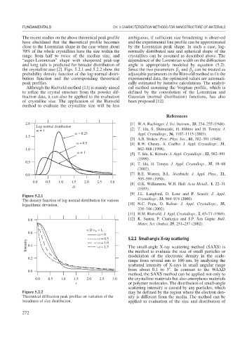
Figure 5.2.1
The density function of log-normal distribution for various Crystallogr., 33, 964–974 (2000).
logarithmic deviation. [10] N.C. Popa, D. Balzar: J. Appl. Crystallogr., 35,
338–346 (2002).
[11] H.M. Rietveld: J. Appl. Crystallogr., 2, 65–71 (1969).
0.8 [12] K. Santra, P. Chatterjee and S.P. Sen Gupta: Bull.
Mater. Sci. (India), 25, 251–257 (2002).
< D > = 1,
0.6 V
= 0
= 0.5 5.2.2 Small-angle X-ray scattering
Intensity 0.4 = 1.0 The small-angle X-ray scattering method (SAXS) is
= 1.5
the method to evaluate the size of small particles or
modulation of the electronic density in the scale-
0.2
range from several nm to 100 nm, by analyzing the
scattered intensity of X-rays in small angular range
from about 0.1 to 5 . In contrast to the WAXD
0.0
method, the SAXS method can be applied not only to
0.0 0.5 1.0 1.5 2.0 2.5 3.0 the crystalline materials but also amorphous materials
s or polymer molecules. The distribution of small-angle
scattering intensity is caused by any particles, which
Figure 5.2.2 may be defined by the region where the electron den-
Theoretical diffraction peak profiles on variation of the sity is different from the media. The method can be
broadness of size distribution. applied to evaluation of the size and distribution of

272