Page 298 - Book Hosokawa Nanoparticle Technology Handbook

5.2 CRYSTAL STRUCTURE FUNDAMENTALS
pores in solid materials [1], local inhomogeneity in
amorphous material, and also colloidal particles and
the coagulation. Analysis of SAXS data is sometimes
aimed at evaluating long-range order or interparticle
distance in collection of polymer molecules by apply-
ing some structure models [2]. Application of SAXS
to evaluate particle size and distribution is described
in this section.
Specially designed optics system should be used for
collecting SAXS data, because accurate evaluation of
small-angle scattering intensities strongly requires
elimination of source X-ray and scattering from the
incident beam path. When laboratory X-ray source is
applied, collimation using curved crystal monochro-
mator, thin slits or small pinholes and precise align-
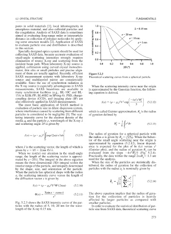
ment of them are usually applied. Recently, efficient Figure 5.2.3
SAXS measurement systems with laboratory X-ray Theoretical scattering curves from a spherical particle.
source and multilayered mirror are commercially
available. Since the use of synchrotron radiation as
the X-ray source is especially advantageous in SAXS When the scattering intensity curve near the origin
measurements, SAXS beamlines are available in is approximated by the Gaussian function, the follow-
many synchrotron facilities (e.g., BL-10C and BL- ing equation is derived,
15A in KEK-PF; BL40B2 in SPring-8). PSD, charge-
coupling device (CCD), and imaging plate (IP) are ⎛ 22 2
sR ⎞
4

also effectively applied in SAXS measurements. Is() ( 0 ) 2 V exp ⎜ g ⎟ (5.2.12)
2
The most basic application of SAXS method is ⎝ 3 ⎠
evaluation of particle size in dilute dispersion system,
where interference caused by scattering from different which is called Guinier approximation. R is the radius
g
particles is considered to be negligible [3]. The scat- of gyration defined by
tering intensity curve for the electron density of the
media and the particle , wavelength of the X-ray 1
0
2
2
and scattering angle 2 is given by R ∫ rdv (5.2.13)
g
V
V
2

)
Is() ( ) 2 ∫ exp ( is r dv (5.2.9) The radius of gyration for a spherical particle with
2

0 the radius a is given by R 3/5a. When the behav-
g
V ior of the small angle scattering near the origin is
approximated by equation (5.2.12), linear depend-
where s is the scattering vector, the length of which is ence is expected for the plot of ln I(s) versus s 2
given by s |s | 2(sin )/ . (Guinier plot), and the radius of gyration R can be
g
2
2
When we restrict our attention in the small-angle evaluated from the slope 4 R /3 (Fig. 5.2.4).
g
range, the length of the scattering vector is approxi- Practically, the data within the range 2 sR 1.3 are
g
mated by s 2 / . The integral in the above equation used for the analysis.
means the three-dimensional (3D) integral within the When the size of the particles are statistically dis-
interior range of the particle, and uniquely determined tributed, the radius of gyration for the collection of
by the shape, size, and orientation of the particle. particles with the radius a is nominally given by
j
When the particle has spherical shape with the radius
a, the scattering intensity curve versus the length of ⎛ 8 ⎞ 1/ 2
the diffraction vector s is given by 3 ∑ a j ⎟
⎜
R ⎜ j 6 ⎟ (5.2.14)
g

2
Is() ( ) 2 V 2 ( sa) (5.2.10) 5 ⎜ ⎝ ∑ a j ⎟ ⎠
2
0 j
3 (sin x x cos )
x
() (5.2.11) The above equation implies that the radius of gyra-
x
x 3 tion for the collection of particles is heavily
affected by larger particles as compared with
Fig. 5.2.3 shows the SAXS intensity curve of the par- smaller particles.
ticles with the radius of 5, 10, 20 nm for the wave- In order to evaluate the statistical distribution of par-
length of the X-ray 0.15 nm. ticle size from SAXS data, theoretical scattering curve
273