Page 299 - Book Hosokawa Nanoparticle Technology Handbook

FUNDAMENTALS CH. 5 CHARACTERIZATION METHODS FOR NANOSTRUCTURE OF MATERIALS
collection are, when the orientations of the particles
are randomly distributed [6]. Therefore, the plot of ln
I(s) versus ln s generally approaches to the straight
line with the slope of 4. Total surface area of the
collection of particles can be evaluated from the scat-
tering intensity curve, if the calibration using a stan-
dard sample with known composition and surface
area is applied.
2
The plot of s I(s) versus the scattering vector s
(Kratky plot) is used to evaluate the shape of the poly-
mer particle, where characteristic change is observed
on transformation from chain-like to granular shape
of particles.

Figure 5.2.4 References
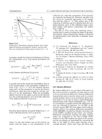
Guinier plot. Theoretical scattering intensity curves from [1] A.V. Semenyuk, D.I. Svergun, L. Yu, Mogilevsky,
spherical particles are plotted by markers, and the solid
2
lines are calculated by Guinier approximation for s 0. V.V. Berezkin, B.V. Mchedlishvili and A.B. Vasilev:
J. Appl. Crystallogr., 24, 809–810 (1991).
[2] T. Veki: The Fourth Series of Experimental Chemistry,
Diffraction, edited by the Chemical Society of Japan,
Vol. 10, Chapter 7, Maruzen Publishing, Tokyo (1992)
assuming a model for statistical distribution is fitted to
the experimental curve. Log-normal distribution [4] (Japanese).
given by [3] A. Guinier: X-ray Diffraction in Crystals, Imperfect
Crystals, and Amorphous Bodies, Chapter 10, Dover
2
1 ⎡ (ln a ln m) ⎤ Publications, New York (1994).
⎢
a m, )
f LN (; exp ⎥ (5.2.15) [4] R. Kranold, S. Kriesen, M. Haselhoff, H.J. Weber
2 ⎣ 2 2 ⎦
a
and G. Goerigk: J. Appl. Crystallogr., 36, 410–414
(2003).
or the Gamma distribution [5] given by [5] W. Ruland, B. Smarsly: J. Appl. Crystallogr., 38, 78–86
(2005).
1 ⎛ a⎞ p 1 ⎛ a⎞ [6] G. Porod: Kolloidn Zh., 124, 83–111 (1951); G. Prod:
fa p
) ⎜ ⎟ exp ⎟ (5.2.16)
(;
,
⎜

p ⎝ ⎠

()
⎝
⎠ Kolloidn Zh., 125, 51–57 (1952); G. Porod: Kolloidn
Zh., 125, 108–122 (1952).
is usually used as the model size distribution. Here m
is the median radius, the logarithmic standard devi-
p 1
ation, (p) t e t dt is the Gamma function, 5.2.3 Neutron diffraction
0
and p and
are the parameters to specify the Gamma
distribution, which give the average p
and the vari- By neutron diffraction, we can obtain information on
2
ance p
for the distribution. When the probability the crystal structure, crystallite size and strain as well
density function of the radius is given by the function as X-ray and electron diffraction. Neutron diffraction
f(a), the scattering intensity curve from the collection measurements need a neutron source such as a reactor
of the spherical particles is given by (steady neutron source) or an accelerator (pulse neu-
tron source) [1]. In case of using a monochromatized
neutron beam with a fixed wavelength (e.g., 1.82 Å),

16 2 it is irradiated to a sample and then the diffraction sig-
Is() ( − 0 ) 2 ∫ a 2 (2 sa f a da (5.2.17)
6
)
)
(
9 nals are collected by detectors. As of 2005, at the
0 research reactor JRR-3M of the Japan Atomic Energy
Agency (JAEA), two neutron diffraction instruments
Porod has shown that the asymptotic behavior at s of the HERMES, installed by Tohoku University, and
of the scattering intensity curve is given by of the HRPD, installed by the JAEA, are working.
Diffraction experiments utilizing the pulse neutron
( ) 2 S source are conducted by the time-of-flight (TOF)
Is () 0 (5.2.18)
8 34 method. In the TOF method, the speed of the neutron
s
and the wavelength are determined by measuring the
where S is the total surface area of the particle, no time of the flight of white pulse neutrons over a
matter what the shape or size distributions of the constant distance. There were Vega and Sirius that
274