Page 55 - Nanotechnology an introduction

etc., all information about the process is completely contained in W , and the process is called purely random.
1
Markov Chains
If, however, the next step of a process depends on its current state, i.e.,

(5.8)
where P denotes the conditional probability that y is in the range (y , y + dy ) after having been at y at an earlier position x, we have a Markov
1
2
2
2
2
chain, defined as a sequence of “trials” (that is, events in which a symbol can be chosen) with possible outcomes a (possible states of the system),
(0)
an initial probability distribution a , and (stationary) transition probabilities defined by a stochastic matrix P. A random sequence, i.e., with a total
absence of correlations between successive symbols, is a zeroth order Markov chain. Without loss of generality we can consider a binary string,
that is a linear sequence of zeros and ones. Such sequences can be generated by choosing successive symbols with a fixed probability. The
probability distribution for an r-step process is
(5.9)
The Markovian transition matrix, if it exists, is a compact way of representing texture.
If upon repeated application of P the distribution a tends to an unchanging limit (i.e., an equilibrial set of states) that does not depend on the initial
state, the Markov chain is said to be ergodic, and

(5.10)
where Q is a matrix with identical rows. Now

(5.11)
and if Q exists it follows, by letting n → ∞, that

(5.12)
from which Q (giving the stationary probabilities, i.e., the equilibrial distribution of a) can be found. Note that if all the transitions of a Markov chain
are equally probable, then there is a complete absence of constraint, in other words the process is purely random.

The entropy of a Markov process is the “average of an average” (i.e., the weighted variety of the transitions). For each row of the (stochastic)
Markov transition matrix, an entropy (Shannon's formula) is computed. The (informational) entropy of the process as a whole is
then the average of these entropies, weighted by the equilibrial distribution of the states.

Runs
Another approach to characterize texture is to make use of the concept of a run, defined as a succession of similar events preceded and
succeeded by different events. Let there again be just two kinds of elements, 0 and 1, and let there be n 0s and n 1s, with n + n = n. r will
0
1
0
0i
1
denote the number of runs of 0 of length i, with , etc. It follows that , etc. Given a set of 0s and 1s, the numbers of different
arrangements of the runs of 0 and 1 are given by multinomial coefficients and the total number of ways of obtaining the set
is [119]
(5.13)

where the terms denoted with square brackets are the multinomial coefficients, which give the number of ways in which n elements can be
partitioned into k subpopulations, the first containing r elements, the second r , etc.:
0
1

(5.14)

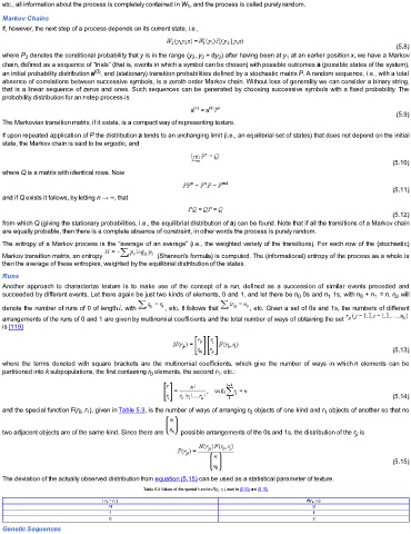
and the special function F(r , r ), given in Table 5.3, is the number of ways of arranging r objects of one kind and r objects of another so that no
1
0 1
0
two adjacent objects are of the same kind. Since there are possible arrangements of the 0s and 1s, the distribution of the r is
ji

(5.15)

The deviation of the actually observed distribution from equation (5.15) can be used as a statistical parameter of texture.
Table 5.3 Values of the special function F(r 0 , r 1 ) used in (5.13) and (5.15)
| r 0 − r 1 | F(r 0 , r 1 )
>1 0
1 1
0 2
Genetic Sequences