Page 54 - Nanotechnology an introduction

encapsulates information about the lateral distribution of the individual roughness components absent in the simple parameters given in Table 5.2:

(5.5)
where the f are the spacial frequencies in the (x, y) plane of the two-dimensional surface profile h(x, y) defined for a square of side L. The power
spectral density is the Fourier transform of the autocorrelation function.
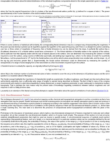
Table 5.2 Table of common roughness parameters. h i is the height of the ith spot on the surface, with reference to some arbitrary fixed level; N is the number of measured spots. Additional parameters are the skew or skewedness (the third
moment of the distribution of h) and the kurtosis (the fourth moment)
Symbol Name Definition Synonyms
Mean height Zeroth moment; d.c. component
Arithmetical mean roughness First moment; centerline average (CLA)
R a
Root mean square roughness Second moment; interface width
R q
Maximum peak to valley Maximum roughness depth
R t
Mean peak to valley height R t averaged over segments
R z
roughness ratio
If there is some evidence of statistical self-similarity, the corresponding fractal dimension may be a compact way of representing the roughness. If
the power spectral density is plotted (as its logarithm) against the logarithm of the spacial frequency, and if there is a straight line portion extending
over two or three orders of magnitude of frequency, then a fractal dimension d can be derived from the slope. A perfectly flat surface has a
C
(Euclidean) dimension of 2; a fractal surface would have a dimension > 2. The formal definition of fractality relates to the capacity of the surface,
and in particular how that capacity scales with the size of objects placed on the surface. One can determine it by measuring the number n of balls
required to cover the surface, using a series of differently sized balls, and plotting log n against log r, where r is the radius of a ball. For a perfectly
2
flat surface, n will be proportional to 1/r , but for the fractal surface one will be able to place proportionally more smaller balls, and the slope −d of
C
the log–log plot becomes greater than 2. Experimentally, the fractal surface dimension could be determined by measuring the quantity of
nanoparticles of a range of sizes ranging from a few nanometers to a few micrometers required to jam the surface.
A fractal dimension is actually the capacity, as originally defined by Kolmogorov [97]:

(5.6)
where N(ε) is the minimum number of p-dimensional cubes of side ε needed to cover the set; p is the dimension of Euclidean space and the set in
question is a bounded subset of that space.
The fractal concept highlights the importance of characteristic length as a parameter of surface roughness, even though very few real surfaces have
self-similarity extending over a sufficiently wide range of lengths to warrant being described as fractals. The fact is that in many of the complex
environments with respect to which biocompatibility is being determined, a single roughness parameter is quite inadequate to characterize surface
topography. That is perhaps the main reason why the present state of knowledge regarding correlations between surface roughness and cell
response is still in a fairly primitive state.
Lacunarity is an extension of the fractal concept that attempts to capture information about the spacial correlations of real surfaces (Section 5.4.3).

5.4.2. One-Dimensional Texture

The techniques discussed in 5.1 and 5.2 are aimed at mapping out the chemical and topographical variegation to as fine a resolution as that of any
variegation that may be present. Raster techniques such as the scanning probe microscopies can identify variegation pixel by pixel and produce a
one-dimensional string of information a priori suitable for analyzing according to the methods suggested in this section (the to-and-fro motion of the
scanning probe may impose a certain kind of correlation on the symbolic sequence if there are two-dimensional features present; i.e., thicker than
a single scanning line). The main task is to determine the presence of compositional and/or topographical correlations within the plane of the
surface.
Preliminary to the discussion of nanotexture proper, which implies a two-dimensional arrangement of features important for molecular and cellular
recognition, let us then consider the one-dimensional situation, which is of course much simpler. The purpose of this section is to look at some
relatively straightforward parameters that might be used as means to quantify texture. A one-dimensional sequence of symbols (each symbol
representing a topographical feature, such as a height, or a chemical element in a particular oxidation state) can be completely defined by the set
of probability distributions W (yx)dy, the probability of finding y, the value of the symbol, in the range (y, y + dy) at position x (if one is moving along
1
the sequence at a uniform rate, this might be equivalent to a time t), W (y x , y x )dy dy , the joint probability of finding y in the range (y , y + dy )
1
2 2
2 1 1
2
1
1
1
at position x and in the range (y , y + dy ) at position x , and so on for triplets, quadruplets and higher multiplets of values of y. If there is an
2
2
1
2
2
unchanging underlying mechanism generating the sequence, the probabilities are stationary and the distributions can be simplified as W (y)dy, the
1
probability of finding y in the range (y, y + dy); W (y y x)dy dy , the joint probability of finding y in the ranges (y , y + dy ) and (y , y + dy ) when
2
2
2
2 1 2
2
1
1
1
1
separated by an interval x = x − x ; etc. If successive values of y are not correlated at all, i.e.,
1
2
(5.7)