Page 180 - Neural Network Modeling and Identification of Dynamical Systems

5.2 SEMIEMPIRICAL ANN-BASED MODEL DESIGN PROCESS 171
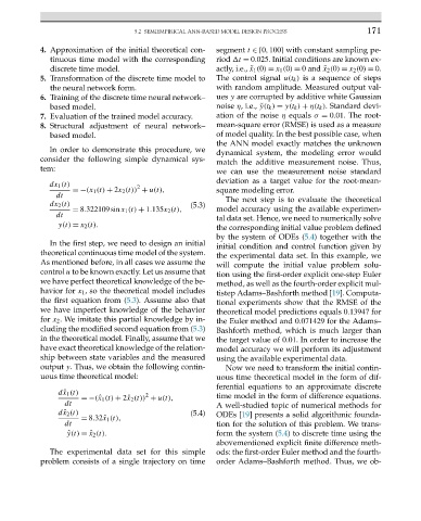
4. Approximation of the initial theoretical con- segment t ∈[0,100] with constant sampling pe-
tinuous time model with the corresponding riod t = 0.025. Initial conditions are known ex-
discrete time model. actly, i.e., ˜x 1 (0) = x 1 (0) = 0 and ˜x 2 (0) = x 2 (0) = 0.
5. Transformation of the discrete time model to The control signal u(t k ) is a sequence of steps
the neural network form. with random amplitude. Measured output val-
6. Training of the discrete time neural network– ues y are corrupted by additive white Gaussian
based model. noise η, i.e., ˜y(t k ) = y(t k ) + η(t k ). Standard devi-
7. Evaluation of the trained model accuracy. ation of the noise η equals σ = 0.01. The root-
8. Structural adjustment of neural network– mean-square error (RMSE) is used as a measure
based model. of model quality. In the best possible case, when
the ANN model exactly matches the unknown
In order to demonstrate this procedure, we
dynamical system, the modeling error would
consider the following simple dynamical sys-
match the additive measurement noise. Thus,
tem: we can use the measurement noise standard
deviation as a target value for the root-mean-
dx 1 (t) 2
=−(x 1 (t) + 2x 2 (t)) + u(t), square modeling error.
dt The next step is to evaluate the theoretical
dx 2 (t) (5.3)
= 8.322109sinx 1 (t) + 1.135x 2 (t), model accuracy using the available experimen-
dt
tal data set. Hence, we need to numerically solve
y(t) = x 2 (t).
the corresponding initial value problem defined
by the system of ODEs (5.4) together with the
In the first step, we need to design an initial
initial condition and control function given by
theoretical continuous time model of the system. the experimental data set. In this example, we
As mentioned before, in all cases we assume the will compute the initial value problem solu-
control u to be known exactly. Let us assume that tion using the first-order explicit one-step Euler
we have perfect theoretical knowledge of the be- method, as well as the fourth-order explicit mul-
havior for x 1 , so the theoretical model includes tistep Adams–Bashforth method [19]. Computa-
the first equation from (5.3). Assume also that tional experiments show that the RMSE of the
we have imperfect knowledge of the behavior theoretical model predictions equals 0.13947 for
for x 2 . We imitate this partial knowledge by in- the Euler method and 0.071429 for the Adams–
cluding the modified second equation from (5.3) Bashforth method, which is much larger than
in the theoretical model. Finally, assume that we the target value of 0.01. In order to increase the
have exact theoretical knowledge of the relation- model accuracy we will perform its adjustment
ship between state variables and the measured using the available experimental data.
output y. Thus, we obtain the following contin- Now we need to transform the initial contin-
uous time theoretical model: uous time theoretical model in the form of dif-
ferential equations to an approximate discrete
d ˆx 1 (t) 2
=−(ˆx 1 (t) + 2ˆx 2 (t)) + u(t), time model in the form of difference equations.
dt A well-studied topic of numerical methods for
d ˆx 2 (t) (5.4) ODEs [19] presents a solid algorithmic founda-
= 8.32ˆx 1 (t),
dt tion for the solution of this problem. We trans-
ˆ y(t) =ˆx 2 (t). form the system (5.4) to discrete time using the
abovementioned explicit finite difference meth-
The experimental data set for this simple ods: the first-order Euler method and the fourth-
problem consists of a single trajectory on time order Adams–Bashforth method. Thus, we ob-