Page 181 - Neural Network Modeling and Identification of Dynamical Systems

172 5. SEMIEMPIRICAL NEURAL NETWORK MODELS OF CONTROLLED DYNAMICAL SYSTEMS

tain the following discrete time counterparts of
the initial theoretical model:
¯ x 1 (t k+1 ) =¯x 1 (t k )

2
+ t −(¯x 1 (t k ) + 2¯x 2 (t k )) + u(t k ) ,
¯ x 2 (t k+1 ) =¯x 2 (t k ) + t [8.32¯x 1 (t k )],
¯ y(t k ) =¯x 2 (t k )
(5.5)

for the Euler method and

2
r 1 (t k ) =−(¯x 1 (t k ) + 2¯x 2 (t k )) + u(t k ),
r 2 (t k ) = 8.32¯x 1 (t k ),
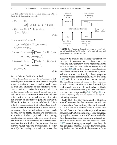
FIGURE 5.1 Canonical form of the recurrent neural net-
t work (From G. Dreyfus. Neural networks: Methodology and
¯ x 1 (t k+4 ) =¯x 1 (t k+3 ) + 55r 1 (t k+3 ) − 59r 1 (t k+2 )
24 applications, Springer-Verlag, 2005).

+ 37r 1 (t k+1 ) − 9r 1 (t k ) ,
necessity to modify the training algorithm for
t
¯ x 2 (t k+4 ) =¯x 2 (t k+3 ) + 55r 2 (t k+3 ) − 59r 2 (t k+2 ) each specific recurrent neural network, we per-
24
form the transformation of the recurrent neural
+ 37r 2 (t k+1 ) − 9r 2 (t k ) ,
network–based models to the unique canonical
¯ y(t k ) =¯x 2 (t k ) form. In [2,20,21], authors propose an algorithm
(5.6) that allows to transform a discrete time dynam-
ical system model defined by a bond graph to
for the Adams–Bashforth method. a corresponding state space model of the form
The theoretical model discretization is fol- (2.13), called the canonical form of the model.
lowed by the transformation of the resulting dif- The resulting canonical form of the recurrent
ference equations into a neural network form. neural network consists of a feedforward lay-
To that end, elements of the difference equa- ered neural network with unit delay feedback
tions are reinterpreted as the respective elements loop that connects some outputs of this network
of the neural network–based model. As a re- with some of its inputs (Fig. 5.1). In Fig. 5.1 and
sult, we obtain a recurrent neural network that in the following, we use the notation z −1 for the
is in one-to-one correspondence with the orig- unit delay element.
inal system of difference equations. However, Note that the abovementioned difficulties
different continuous time models lead to differ- arise if we consider the recurrent neural net-
ent difference equations that, in turn, lead to dif- works derived from arbitrary discrete time mod-
ferent recurrent neural network–based models. els. If we consider instead only the networks
In general, these neural network–based mod- derived from the discrete time approximations
els may have a highly diverse and complicated of systems of ODEs in the normal form provided
architecture. A direct approach to the training by explicit one-step finite difference methods,
problem for such neural networks would in gen- then the resulting recurrent neural network ar-
eral require the development of different train- chitecture immediately has the canonical form
ing algorithms, suited for the corresponding re- (2.13). Also, if we apply an explicit multistep fi-
current neural network architectures. In order nite difference method, the only transformation
to unify the training approach and avoid the required to put the model in the canonical form