Page 186 - Neural Network Modeling and Identification of Dynamical Systems

5.3 SEMIEMPIRICAL ANN-BASED MODEL DERIVATIVES COMPUTATION 177
TABLE 5.1 Model prediction error for each stage of model design.
Theory ANN-1 ANN-2 ANN-3 Empir
Euler 0.13947 0.13593 0.12604 0.01394 –
Adams–Bashforth 0.07143 0.07104 0.03883 0.01219 –
NARX – – – – 0.02821

“Empir” signifies the best results for the empiri-
cal NARX model of the system.

5.3 SEMIEMPIRICAL ANN-BASED
MODEL DERIVATIVES
COMPUTATION

Semiempirical neural network–based models
of the form (5.2) are continuous time models, in
contrast to discrete time purely empirical mod-
els, described in Chapter 2; hence the training
methods for these models are also formulated
in continuous time. Despite the fact that the
actual implementation of these algorithms re-
quires the appropriate finite difference approx-
imations of the ODEs, the continuous time algo-
rithm versions provide an additional flexibility
in the choice of the most suitable finite difference
method. The total error function E : R n w → R
¯
evaluated on the training set of the form (5.1)is
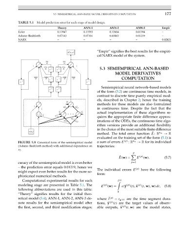
FIGURE 5.9 Canonical form of the semiempirical model asumof errors E (p) : R n w → R for its individual
(Adams–Bashforth method) with additional dependence on trajectories:
x 2 .
P
(p)
¯
E(w) = E (w). (5.7)
curacy of the semiempirical model is even better p=1
– the prediction error equals 0.01219, hence we (p)
The individual errors E have the following
might expect even better results for the more so-
form:
phisticated numerical methods.
Computational experimental results for each ¯ t (p)

modeling stage are presented in Table 5.1.The E (p) (w) = e(˜y (p) (t), ˆ x (p) (t,w),w)dt, (5.8)
following abbreviations are used in this table:
0
“Theory” signifies results for the initial theo-
retical model (5.4); ANN-1, ANN-2, ANN-3 de- where ¯ t (p) = t K (p) are the time segment dura-
note results for the semiempirical model after tions, ˜y (p) (t) are the target values of observ-
the first, second, and third modification stages; able outputs, ˆ x (p) (t,w) are the model states,