Page 187 - Neural Network Modeling and Identification of Dynamical Systems

178 5. SEMIEMPIRICAL NEURAL NETWORK MODELS OF CONTROLLED DYNAMICAL SYSTEMS

and e (p) : R n y × R n x × R n w → R represent the derivatives: one method operates forward-in-
model prediction error at time instant t. Under time, and the other operates backward-in-time.
the usual assumptions of the additive Gaussian We begin with a description of a continuous
white measurement noise, it seems reasonable to time counterpart of a forward-in-time RTRL al-
utilize the instantaneous error function e of the gorithm.
following form: The gradient of the individual trajectory error
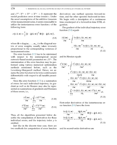
function (5.8) equals
1 T
e(˜y, ˆ x,w) = ˜ y − ˆ g(ˆ x,w) ˜y − ˆ g(ˆ x,w) ,
2 ¯ t

(5.9) ∂E(w) ∂e(˜y(t), ˆ x(t,w),w)
=
∂w ∂w
) is the diagonal ma- 0
where = diag(ω 1 ,...,ω n y T
trix of error weights, usually taken inversely ∂ ˆ x(t,w) ∂e(˜y(t), ˆ x(t,w),w)
+ dt,
proportional to the corresponding variances of ∂w ∂ ˆ x
measurement noise. (5.12)
The error function (5.7) has to be minimized
with respect to the semiempirical neural and its Hessian equals
network–based model parameters w ∈ R .The
n w
minimization of the error function may be per- ¯ t
2
2
∂ E(w) ∂ e(˜y(t), ˆ x(t,w),w)
formed using various numerical optimization =
methods mentioned before, such as the ∂w 2 ∂w 2
0
Levenberg–Marquardt method. Hence, we as- 2
sume the error function to be twice continuously + ∂ e(˜y(t), ˆ x(t,w),w) ∂ ˆ x(t,w)
differentiable with respect to all tunable param- ∂w∂ ˆ x ∂w
T 2
eters. ∂ ˆ x(t,w) ∂ e(˜y(t), ˆ x(t,w),w)
+
Since the error function (5.7) is a summation ∂w ∂ ˆ x∂w
of errors for each individual trajectory, its gra- ∂ ˆ x(t,w) ∂ e(˜y(t), ˆ x(t,w),w) ∂ ˆ x(t,w)
T
2
dient as well as its Hessian may also be repre- + ∂w ∂ ˆ x 2 ∂w
sented as summations of gradients and Hessians n x 2
∂e(˜y(t), ˆ x(t,w),w) ∂ ˆ x i (t,w)
of these errors, i.e., + dt.
∂ ˆ x i ∂w 2
i=1
P (p)
¯
∂E(w) ∂E (w) (5.13)
= , (5.10)
∂w ∂w
p=1
First-order derivatives of the instantaneous er-
P 2 (p)
∂ E(w) ∂ E (w) ror function (5.9) have the form
2 ¯
= . (5.11)
∂w 2 ∂w 2
p=1 T
∂e(˜y, ˆ x,w) ∂ ˆ g(ˆ x,w)
=− ˜y − ˆ g(ˆ x,w) ,
Thus, all the algorithms presented below de- ∂w ∂w
T
scribe the computation of derivatives for these ∂e(˜y, ˆ x,w) ∂ ˆ g(ˆ x,w)
=− ˜y − ˆ g(ˆ x,w) ,
individual errors, and the trajectory index p is ∂ ˆ x ∂ ˆ x
omitted. (5.14)
Just like in the discrete time case, there are
two methods for computation of error function and its second-order derivatives are