Page 213 - Neural Network Modeling and Identification of Dynamical Systems

204 6. NEURAL NETWORK SEMIEMPIRICAL MODELING OF AIRCRAFT MOTION

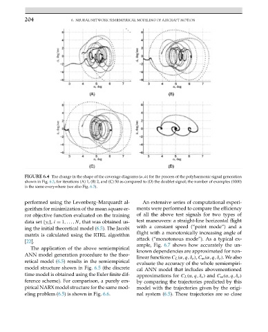
FIGURE 6.4 The change in the shape of the coverage diagrams (α, ˙α) for the process of the polyharmonic signal generation
shown in Fig. 6.3, for iterations (A) 1, (B) 2, and (C) 50 as compared to (D) the doublet signal; the number of examples (1000)
is the same everywhere (see also Fig. 6.3).

performed using the Levenberg–Marquardt al- An extensive series of computational experi-
gorithm for minimization of the mean square er- ments were performed to compare the efficiency
ror objective function evaluated on the training of all the above test signals for two types of
data set {y i }, i = 1,...,N, that was obtained us- test maneuvers: a straight-line horizontal flight
ing the initial theoretical model (6.5). The Jacobi with a constant speed (“point mode”) and a
flight with a monotonically increasing angle of
matrix is calculated using the RTRL algorithm
attack (“monotonous mode”). As a typical ex-
[22].
ample, Fig. 6.7 shows how accurately the un-
The application of the above semiempirical
known dependencies are approximated for non-
ANN model generation procedure to the theo-
linear functions C L (α,q,δ e ), C m (α,q,δ e ).Wealso
retical model (6.5) results in the semiempirical
evaluate the accuracy of the whole semiempiri-
model structure shown in Fig. 6.5 (the discrete cal ANN model that includes abovementioned
time model is obtained using the Euler finite dif- approximations for C L (α,q,δ e ) and C m (α,q,δ e )
ference scheme). For comparison, a purely em- by comparing the trajectories predicted by this
pirical NARX model structure for the same mod- model with the trajectories given by the origi-
eling problem (6.5) is shown in Fig. 6.6. nal system (6.5). These trajectories are so close