Page 222 - Neural Network Modeling and Identification of Dynamical Systems

6.3 SEMIEMPIRICAL MODELING OF AIRCRAFT THREE-AXIS ROTATIONAL MOTION 213
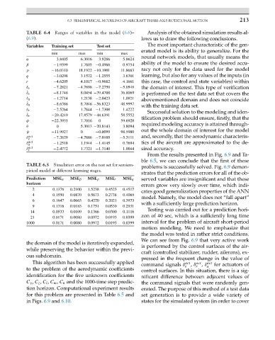
TABLE 6.4 Ranges of variables in the model (6.6)– Analysis of the obtained simulation results al-
(6.9). lows us to draw the following conclusions.
Variables Training set Test set The most important characteristic of the gen-
erated model is its ability to generalize. For the
min max min max
neural network models, that usually means the
α 3.8405 6.3016 3.9286 5.8624
ability of the model to ensure the desired accu-
β −1.9599 1.7605 −0.4966 0.9754
racy not only for the data used for the model
p −16.0310 18.1922 −10.1901 11.8683
q −3.0298 3.1572 −1.2555 3.6701 learning, but also for any values of the inputs (in
r −4.6205 4.1017 −0.9682 4.1661 this case, the control and state variables) within
δ e −7.2821 −4.7698 −7.2750 −5.0549 the domain of interest. This type of verification
˙ δ e −8.1746 8.0454 −39.4708 36.8069 is performed on the test data set that covers the
δ a −1.2714 1.2138 −2.0423 1.0921 abovementioned domain and does not coincide
˙ δ a −8.6386 8.7046 −56.8323 48.9997
with the training data set.
δ r −2.5264 1.7844 −1.7308 1.4222
Successful solution to the modeling and iden-
˙ δ r −20.4249 17.8579 −48.6391 58.5552
tification problem should ensure, firstly, that the
φ −22.3955 7.7016 0 59.6928
required modeling accuracy is attained through-
θ 0 5.3013 −20.8143 3.8094
out the whole domain of interest for the model
ψ −11.9927 0 −0.0099 98.5980
δ e act −7.2629 −4.7886 −7.0105 −5.3111 and, secondly, that the aerodynamic characteris-
δ a act −1.2518 1.1944 −1.4145 0.7694 tics of the aircraft are approximated to the de-
δ r act −2.4772 1.7321 −1.3140 1.0044 sired accuracy.
From the results presented in Fig. 6.9 and Ta-
ble 6.5, we can conclude that the first of these
TABLE 6.5 Simulation error on the test set for semiem- problems is successfully solved. Fig. 6.9 demon-
pirical model at different learning stages.
strates that the prediction errors for all of the ob-
Prediction MSE α MSE β MSE p MSE r MSE q served variables are insignificant and that these
horizon errors grow very slowly over time, which indi-
2 0.1376 0.2100 1.5238 0.4523 0.4517
cates good generalization properties of the ANN
4 0.1550 0.0870 0.5673 0.2738 0.4069
model. Namely, the model does not “fall apart”
6 0.1647 0.0663 0.4270 0.2021 0.3973
with a sufficiently large prediction horizon.
9 0.1316 0.0183 0.1751 0.0530 0.2931
Testing was carried out for a prediction hori-
14 0.0533 0.0109 0.1366 0.0300 0.1116
zon of 40 sec, which is a sufficiently long time
21 0.0171 0.0080 0.0972 0.0193 0.0399
1000 0.0171 0.0080 0.0972 0.0193 0.0399 interval for the problem of aircraft short-period
motion modeling. We need to emphasize that
the model was tested in rather strict conditions.
We can see from Fig. 6.9 that very active work
the domain of the model is iteratively expanded,
is performed by the control surfaces of the air-
while preserving the behavior within the previ-
craft (controlled stabilizer, rudder, ailerons), ex-
ous subdomain.
pressed in the frequent change in the value of
This algorithm has been successfully applied act act act
command signals δ e , δ r , δ a for actuators of
to the problem of the aerodynamic coefficients control surfaces. In this situation, there is a sig-
identification for the five unknown coefficients nificant difference between adjacent values of
C y , C z , C l , C m , C n and the 1000-time step predic- the command signals that were randomly gen-
tion horizon. Computational experiment results erated. The purpose of this method of a test data
for this problem are presented in Table 6.5 and set generation is to provide a wide variety of
in Figs. 6.9 and 6.10. states for the simulated system (in order to cover