Page 226 - Neural Network Modeling and Identification of Dynamical Systems

6.4 SEMIEMPIRICAL MODELING OF AIRCRAFT LONGITUDINAL TRANSLATIONAL AND ANGULAR MOTION 217
output up to any preassigned accuracy. One pur- characterizing the accuracy of the generated
pose of this section is to verify the validity of ANN model as a whole are given as well as
this hypothesis concerning a somewhat compli- the efficiency of solving the problem of iden-
cated applied problem. We consider the prob- tifying the aerodynamic characteristics of the
lem of extracting the dependencies for the coef- aircraft.
ficients C x , C z , C m from the experimental data To solve this problem, we need to develop a
for a rather wide range of possible values of mathematical model of the longitudinal motion
their arguments, typical for a maneuverable air- of the aircraft. In this case we consider a system
craft. As is well known [22], in order to obtain of nonlinear ODEs traditional for aircraft flight
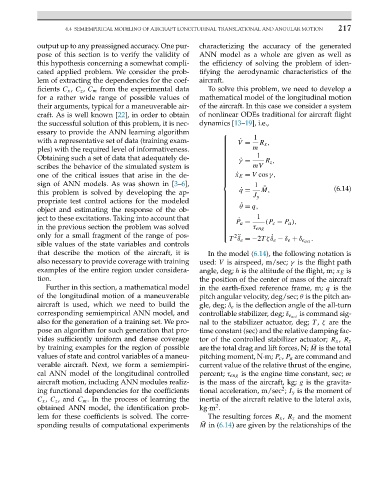
the successful solution of this problem, it is nec- dynamics [13–19], i.e.,
essary to provide the ANN learning algorithm ⎧
with a representative set of data (training exam- ⎪ V = 1 R x ,
˙
⎪
⎪
ples) with the required level of informativeness. ⎪ m
⎪
⎪
⎪
Obtaining such a set of data that adequately de- ⎪ 1
⎪
⎪
⎪ ˙ γ = R z ,
scribes the behavior of the simulated system is ⎪ mV
⎪
⎪
⎪
⎪
one of the critical issues that arise in the de- ⎪ x E = V cosγ,
˙
⎪
⎪
sign of ANN models. As was shown in [3–6], ⎨ 1 ¯ (6.14)
this problem is solved by developing the ap- ⎪ ˙ q = M,
⎪ J y
propriate test control actions for the modeled ⎪
⎪
⎪
˙
⎪ θ = q,
object and estimating the response of the ob- ⎪
⎪
⎪
⎪
ject to these excitations. Taking into account that ⎪ ˙ 1
⎪
⎪
⎪ P a = (P c − P a ),
in the previous section the problem was solved ⎪ τ eng
⎪
⎪
⎪
only for a small fragment of the range of pos- ⎪ 2 ¨ ˙
⎩
T δ e =−2Tζδ e − δ e + δ e act .
sible values of the state variables and controls
that describe the motion of the aircraft, it is In the model (6.14), the following notation is
also necessary to provide coverage with training used: V is airspeed, m/sec; γ is the flight path
examples of the entire region under considera- angle, deg; h is the altitude of the flight, m; x E is
tion. the position of the center of mass of the aircraft
Further in this section, a mathematical model in the earth-fixed reference frame, m; q is the
of the longitudinal motion of a maneuverable pitch angular velocity, deg/sec; θ is the pitch an-
aircraft is used, which we need to build the gle, deg; δ e is the deflection angle of the all-turn
corresponding semiempirical ANN model, and is command sig-
controllable stabilizer, deg; δ e act
also for the generation of a training set. We pro- nal to the stabilizer actuator, deg; T , ζ are the
pose an algorithm for such generation that pro- time constant (sec) and the relative damping fac-
vides sufficiently uniform and dense coverage tor of the controlled stabilizer actuator; R x , R z
by training examples for the region of possible are the total drag and lift forces, N; M is the total
¯
values of state and control variables of a maneu- pitching moment, N·m; P c , P a are command and
verable aircraft. Next, we form a semiempiri- current value of the relative thrust of the engine,
cal ANN model of the longitudinal controlled percent; τ eng is the engine time constant, sec; m
aircraft motion, including ANN modules realiz- is the mass of the aircraft, kg; g is the gravita-
2
ing functional dependencies for the coefficients tional acceleration, m/sec ; I y is the moment of
C x , C z ,and C m . In the process of learning the inertia of the aircraft relative to the lateral axis,
2
obtained ANN model, the identification prob- kg·m .
lem for these coefficients is solved. The corre- The resulting forces R x , R z and the moment
sponding results of computational experiments M in (6.14) are given by the relationships of the
¯