Page 59 - Neural Network Modeling and Identification of Dynamical Systems

2.1 ARTIFICIAL NEURAL NETWORK STRUCTURES 47

FIGURE 2.18 Nonlinear AutoRegressive network with eXogeneous inputs.

The input–output modeling approach has seri-
ous drawbacks: first, the minimum time win-
dow size required to achieve the desired accu-
racy is not known beforehand; second, in order
to learn the long-term dependencies one might
need an arbitrarily large time window; third, if a
dynamical system is nonstationary, the optimal
time window size might change over time.
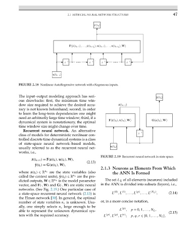
Recurrent neural network. An alternative
class of models for deterministic nonlinear con-
trolled discrete time dynamical systems is a class
of state-space neural network–based models,
usually referred to as the recurrent neural net-
works, i.e.,
FIGURE 2.19 Recurrent neural network in state space.
z(t k+1 ) = F(z(t k ),u(t k ),W),
(2.13)
ˆ y(t k ) = G(z(t k ),W),
2.1.3 Neurons as Elements From Which
where z(t k ) ∈ R n z are the state variables (also the ANN Is Formed
called the context units), ˆy(t k ) ∈ R n y are the pre-
dicted outputs, W ∈ R n w is the model parameter The set L of all elements (neurons) included
vector, and F(·,W) and G(·,W) are static neural in the ANN is divided into subsets (layers), i.e.,
networks. (See Fig. 2.19.) One particular case of
(1)
(0)
a state-space recurrent neural network (2.13)is L ,L ,...,L (p) ,...,L (N L ) , (2.14)
the Elman network [30]. In general, the optimal
number of state variables n z is unknown. Usu- or, in a more concise notation,
ally, one simply selects n z large enough to be (p)
L , p = 0,1,...,N L ,
able to represent the unknown dynamical sys- (2.15)
(r)
tem with the required accuracy. L (p) ,L (q) ,L ; p,q,r ∈{0,1,...,N L },