Page 207 - Numerical Analysis Using MATLAB and Excel

Chapter 5 Differential Equations, State Variables, and State Equations

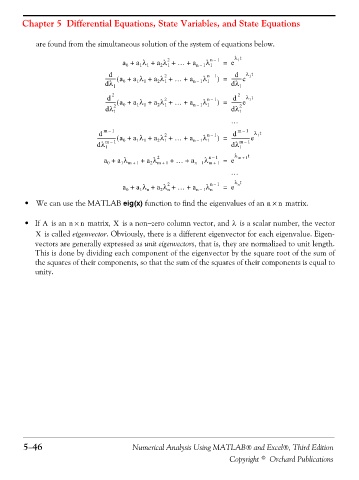
are found from the simultaneous solution of the system of equations below.

2
1
a + a λ + a λ + … + a n – 1 λ n – 1 = e λ t
1
0
1
1
1
2
d d λ t
2
--------- a +( a λ + a λ + … + a λ n – 1 ) = --------e 1
dλ 1 0 1 1 2 1 n – 1 1 dλ 1
2
d
2
-------- a +( d 2 0 a λ + a λ + … + a n – 1 λ n – 1 ) = --------e λ t
1
1
1
2
1
1
dλ 2 1 dλ 2 1
…
m –
1
d
2
--------------- a +( d m – 1 0 a λ + a λ + … + a n – 1 λ n – 1 ) = ---------------e λ t
1
1
2
1
1
1
dλ m – 1 dλ m – 1
1
1
a + a λ m + 1 + a λ 2 m + 1 + … + a n – 1 λ n – 1 1 = e λ m + 1 t
1
2
0
m +
…
2
n
a + a λ + a λ + … + a n – 1 λ n – 1 = e λ t
n
n
2
0
1
n
• We can use the MATLAB eig(x) function to find the eigenvalues of an n × n matrix.
• If is an n × n matrix, is a non−zero column vector, and is a scalar number, the vector
λ
X
A
X is called eigenvector. Obviously, there is a different eigenvector for each eigenvalue. Eigen-
vectors are generally expressed as unit eigenvectors, that is, they are normalized to unit length.
This is done by dividing each component of the eigenvector by the square root of the sum of
the squares of their components, so that the sum of the squares of their components is equal to
unity.

5−46 Numerical Analysis Using MATLAB® and Excel®, Third Edition

Copyright © Orchard Publications