Page 205 - Numerical Analysis Using MATLAB and Excel

Chapter 5 Differential Equations, State Variables, and State Equations

ters. This method will work with all linear equations including those with variable coefficients
provided that the general form of the natural response is known.
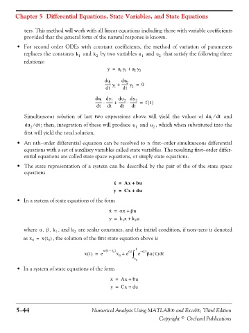
• For second order ODEs with constant coefficients, the method of variation of parameters
replaces the constants k 1 and k 2 by two variables u 1 and u 2 that satisfy the following three
relations:
y = u y + u y
2 2
1 1
du du
1
2
------- y + -------- y = 0
dt 1 dt 2
du dy du dy
1
2
2
1
⋅
⋅
-------- -------- + -------- -------- = ft()
dt dt dt dt
⁄
Simultaneous solution of last two expressions above will yield the values of du dt and
1
du ⁄ dt ; then, integration of these will produce u 1 and u 2 , which when substituted into the
2
first will yield the total solution.
•An nth−order differential equation can be resolved to first−order simultaneous differentialn
equations with a set of auxiliary variables called state variables. The resulting first−order differ-
ential equations are called state space equations, or simply state equations.
• The state representation of a system can be described by the pair of the of the state space
equations

·
x = Ax + bu
y = Cx + du

• In a system of state equations of the form
·
x = αx + βu
y = k x + k u
2
1
where , , αβ k 1 , and k 2 are scalar constants, and the initial condition, if non−zero is denoted
as x = xt() , the solution of the first state equation above is
0
0
(
α t – t ) 0 αt t – ατ
d
xt() = e x + e ∫ e βu τ() τ
0
t 0
• In a system of state equations of the form
·
x = Ax + bu
y = Cx + du

5−44 Numerical Analysis Using MATLAB® and Excel®, Third Edition

Copyright © Orchard Publications