Page 201 - Numerical Analysis Using MATLAB and Excel

Chapter 5 Differential Equations, State Variables, and State Equations

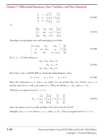
5 7 – 5 x 1 x 1
0 4 – 1 x 2 = λ x 2 (5.162)
2 8 – 3 x x
3 3
or
5x 1 7x 2 – 5x 3 λx 1

0 4x 2 – x 3 = λx 2 (5.163)
2x 1 8x 2 – 3x 3 λx 3

Equating corresponding rows and rearranging, we obtain

)
( 5 – λ x 1 7x 2 – 5x 3 0
)
–
0 ( 4 λ x 2 – x 3 = 0 (5.164)
2x 1 8x 2 ( 3 λ x 3 0
) –
–
For λ = 1 , (5.164) reduces to
4x + 7x – 5x = 0
2
3
1
3x – x = 0 (5.165)
2
3
2x + 8x – 4x = 0
3
1
2
By Crame’s rule, or MATLAB, we obtain the indeterminate values
⁄
x = 00 x = 00 x = 00 (5.166)
⁄
⁄
3
2
1
,
,
Since the unknowns x x and x 3 are scalars, we can assume that one of these, say x 2 , is
1
2
known, and solve x 1 and x 3 in terms of x 2 . Then, we obtain x = 2x 2 , and x = 3x 2 .
3
1
Therefore, an eigenvector for λ = 1 is
x 1 2x 2 2 2
X λ = 1 = x 2 = x 2 = x 2 1 = 1 (5.167)
x 3 3x 2 3 3
since any eigenvector is a scalar multiple of the last vector in (5.167).
Similarly, for λ = 2 , we obtain x = x 2 , and x = 2x 2 . Then, an eigenvector for λ = 2 is
3
1

5−40 Numerical Analysis Using MATLAB® and Excel®, Third Edition

Copyright © Orchard Publications