Page 199 - Numerical Analysis Using MATLAB and Excel

Chapter 5 Differential Equations, State Variables, and State Equations

5.11 Eigenvectors

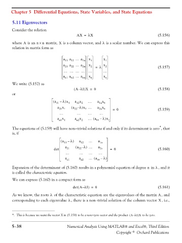
Consider the relation
AX = λX (5.156)

where is an n × n matrix, is a column vector, and is a scalar number. We can express this
λ
X
A
relation in matrix form as
a 11 a 12 … a 1n x 1 x 1
a 21 a 22 … a 2n x 2 = λ x 2 (5.157)
…… … … … …
a n1 a n2 … a nn x n x n
We write (5.157) as
( A λI X = 0 (5.158)
)
–
or
)
a ( 11 – λ x 1 a x … a x
1n n
12 2
)
a x ( a – λ x … a x = 0 (5.159)
2n n
22
21 1
2
… … … …
)
(
a x a x … a – λ x n
n2 2
nn
n1 1
*
The equations of (5.159) will have non−trivial solutions if and only if its determinant is zero , that
is, if
a ( 11 – λ ) a 12 … a 1n
a ( a – λ … ) a
det 21 22 2n = 0 (5.160)
… … … …
(
a n1 a n2 … a – λ )
nn
Expansion of the determinant of (5.160) results in a polynomial equation of degree in , and it
λ
n
is called the characteristic equation.
We can express (5.160) in a compact form as
(
)
det A λI = 0 (5.161)
–
As we know, the roots of the characteristic equation are the eigenvalues of the matrix , and
λ
A
corresponding to each eigenvalue , there is a non−trivial solution of the column vector , i.e.,
λ
X
)
(
*. This is because we want the vector X in (5.158) to be a non−zero vector and the product A λI X to be zero.
–
5−38 Numerical Analysis Using MATLAB® and Excel®, Third Edition

Copyright © Orchard Publications