Page 197 - Numerical Analysis Using MATLAB and Excel

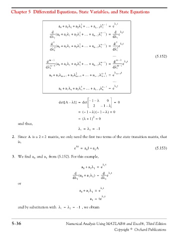
Chapter 5 Differential Equations, State Variables, and State Equations

2
1
a + a λ + a λ + … + a n – 1 λ n – 1 = e λ t
1
1
0
2
1
1
d
2
--------- a +( d a λ + a λ + … + a λ n – 1 ) = --------e λ t
1
dλ 1 0 1 1 2 1 n – 1 1 dλ 1
2
d
2
1
-------- a +( d 2 a λ + a λ + … + a λ n – 1 ) = --------e λ t
dλ 2 1 0 1 1 2 1 n – 1 1 dλ 2 1
… (5.152)
d m – 1 d m – 1 λ t
2
--------------- a +( 0 a λ + a λ + … + a n – 1 λ n – 1 ) = ---------------e 1
1
1
1
1
2
dλ m – 1 dλ m – 1
1
1
a + a λ m + 1 + a λ 2 m + 1 + … + a n – 1 λ n – 1 1 = e λ m + 1 t
m +
1
0
2
…
2
n
a + a λ + a λ + … + a n – 1 λ n – 1 = e λ t
n
1
0
2
n
n
[
]
–
det A λI = det – 1 – λ 0 = 0
2 – 1 – λ
)
)
(
–
= – ( 1 λ – – λ = 0
1
= ( λ + 1 ) 2 = 0
and thus,
λ = λ = – 1
1
2
2. Since is a 2 × 2 matrix, we only need the first two terms of the state transition matrix, that
A
is,
e At = a I + a A (5.153)
1
0
3. We find a 0 and a 1 from (5.152). For this example,
λ t
a + a λ = e 1
0
1 1
d
--------- a +( d a λ ) = ---------e λ t
1
dλ 1 0 1 1 dλ 1
or
λ t
1
a + a λ = e
0
1 1
λ t
1
a = te
1
and by substitution with λ = λ = – 1 , we obtain
1
2
5−36 Numerical Analysis Using MATLAB® and Excel®, Third Edition
Copyright © Orchard Publications