Page 196 - Numerical Analysis Using MATLAB and Excel

Computation of the State Transition Matrix

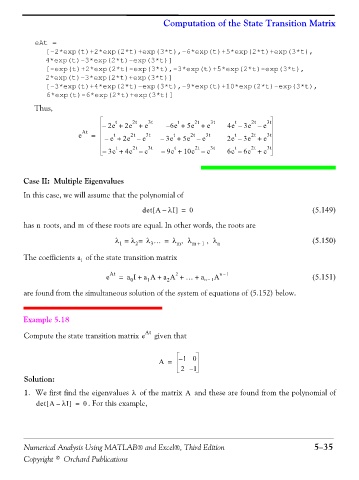
eAt =
[-2*exp(t)+2*exp(2*t)+exp(3*t),-6*exp(t)+5*exp(2*t)+exp(3*t),
4*exp(t)-3*exp(2*t)-exp(3*t)]
[-exp(t)+2*exp(2*t)-exp(3*t),-3*exp(t)+5*exp(2*t)-exp(3*t),
2*exp(t)-3*exp(2*t)+exp(3*t)]
[-3*exp(t)+4*exp(2*t)-exp(3*t),-9*exp(t)+10*exp(2*t)-exp(3*t),
6*exp(t)-6*exp(2*t)+exp(3*t)]
Thus,

2t
2t
t
t
2t
t
– 2e + 2e + e 3t – 6e + 5e + e 3t 4e – 3e – e 3t
At
e = – e + 2e – e 3t – 3e + 5e – e 3t 2e – 3e + e 3t
t
2t
t
2t
t
2t
2t
t
2t
2t
t
t
– 3e + 4e – e 3t – 9e + 10e – e 3t 6e – 6e + e 3t
Case II: Multiple Eigenvalues
In this case, we will assume that the polynomial of
]
[
det A λI = 0 (5.149)
–
has roots, and of these roots are equal. In other words, the roots are
m
n
λ = λ = λ … 3 λ = m , λ m + 1 , λ n (5.150)
1
2
The coefficients of the state transition matrix
a
i
2
e At = a I + a A + a A + … + a n – 1 A n – 1 (5.151)
0
2
1
are found from the simultaneous solution of the system of equations of (5.152) below.
Example 5.18
At
Compute the state transition matrix e given that
A = – 1 0
2 – 1
Solution:
1. We first find the eigenvalues of the matrix and these are found from the polynomial of
λ
A
]
[
det A λI = 0 . For this example,
–

Numerical Analysis Using MATLAB® and Excel®, Third Edition 5−35

Copyright © Orchard Publications