Page 191 - Numerical Analysis Using MATLAB and Excel

Chapter 5 Differential Equations, State Variables, and State Equations

Then,
(
·
At –
d
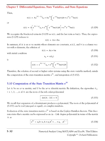
x t() = Ae At – t ) 0 x + Ae At ∫ t e – Aτ bu τ() τ + e e At bu t()
0
t 0
or
(
·
At –
x t() = Ae At – t ) 0 x + e At ∫ t e – Aτ bu τ() τ + e e At bu t() (5.129)
d
0
t 0
We recognize the bracketed terms in (5.129) as xt() , and the last term as bu t() . Thus, the expres-
sion (5.129) reduces to
·
x t() = Ax + bu
In summary, if is an n × n matrix whose elements are constants, n ≥ 2 , and is a column vec-
A
b
tor with n elements, the solution of
·
x t() = Ax + bu (5.130)
with initial condition
x = xt() (5.131)
0
0
is
(
At – t ) 0 At t – Aτ
d
xt() = e x + e ∫ e bu τ() τ (5.132)
0
t 0
Therefore, the solution of second or higher order systems using the state variable method, entails
the computation of the state transition matrix e At , and integration of (5.132).

5.10 Computation of the State Transition Matrix e At

Let be an n × n matrix, and be the n × I n identity matrix. By definition, the eigenvalues λ i ,
A
,
,,
i = 1 2 … n of are the roots of the nth order polynomial
A
[
]
det A – λI = 0 (5.133)
We recall that expansion of a determinant produces a polynomial. The roots of the polynomial of
(5.133) can be real (unequal or equal), or complex numbers.

Evaluation of the state transition matrix e At is based on the Cayley−Hamilton theorem. This theo-
)
(
rem states that a matrix can be expressed as an n – 1 th degree polynomial in terms of the matrix
A as
At 2 n – 1
e = a I + a A + a A + … + a n – 1 A (5.134)
2
1
0
5−30 Numerical Analysis Using MATLAB® and Excel®, Third Edition

Copyright © Orchard Publications