Page 192 - Numerical Analysis Using MATLAB and Excel

Computation of the State Transition Matrix

λ
where the coefficients are functions of the eigenvalues . We accept (5.134) without proving
a
i
it. The proof can be found in Linear Algebra and Matrix Theory textbooks.
Since the coefficients are functions of the eigenvalues , we must consider the following cases:
λ
a
i
Case I: Distinct Eigenvalues (Real or Complex)
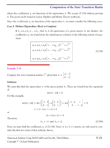
If λ ≠ 1 λ ≠ 2 λ ≠ 3 … λ ≠ n , that is, if all eigenvalues of a given matrix A are distinct, the

coefficients are found from the simultaneous solution of the following system of equa-
a
i
tions:

2 n – 1 λ t
1
a + a λ + a λ + … + a n – 1 λ 1 = e
2
1
1
0
1
2
2
a + a λ + a λ + … + a n – 1 λ n – 1 = e λ t (5.135)
0
2
2
1
2
2
…
2
λ
n
a + a λ + a λ + … + a n – 1 n n – 1 = e λ t
2 n
1 n
0
Example 5.16
At – 2 1
Compute the state transition matrix e given that A =
0 – 1
Solution:
We must first find the eigenvalues of the given matrix . These are found from the expansion
λ
A
of
[
]
det A λI = 0
–
For this example,
⎧ – 2 1 10 ⎫ – 2 – λ 1
[
]
det A λI = det ⎨ – λ ⎬ = det = 0
–
⎩ 0 – 1 01 ⎭ 0 – 1 λ
–
)
)
(
= – ( 2 – λ – 1 – λ = 0
or
( λ + 1 λ ) ( + 2 = 0
)
Therefore,
λ = – 1 and λ = – 2 (5.136)
1
2
Next, we must find the coefficients of (5.134). Since is a 2 × 2 matrix, we only need to con-
A
a
i
sider the first two terms of that relation, that is,
Numerical Analysis Using MATLAB® and Excel®, Third Edition 5−31
Copyright © Orchard Publications