Page 188 - Numerical Analysis Using MATLAB and Excel

Solution of Single State Equations

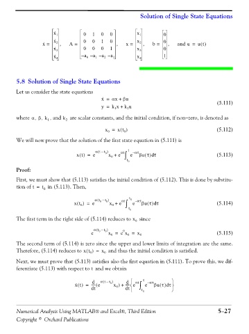
x · 1 0 1 0 0 x 1 0
·
x = x · 2 , A = 0 0 1 0 , x = x 2 , b = 0 , and u = ut()
x · 3 0 0 0 1 x 3 0
x · 4 a – 0 a – 1 a – 2 a – 3 x 4 1

5.8 Solution of Single State Equations

Let us consider the state equations
·
x = αx + βu (5.111)
y = k x + k u
2
1
where , , αβ k 1 , and k 2 are scalar constants, and the initial condition, if non−zero, is denoted as

x = xt() (5.112)
0
0
We will now prove that the solution of the first state equation in (5.111) is

(
α t – t ) αt t – ατ
xt() = e 0 x + e ∫ e βu τ() τ (5.113)
d
0
t 0
Proof:
First, we must show that (5.113) satisfies the initial condition of (5.112). This is done by substitu-
tion of t = t 0 in (5.113). Then,

t
(
α t – t ) 0 αt 0 – ατ
0
d
xt () = e x + e ∫ e βu τ() τ (5.114)
0
0
t 0
The first term in the right side of (5.114) reduces to x 0 since
α t – t ) 0 0
(
0
e x = e x = x 0 (5.115)
0
0
The second term of (5.114) is zero since the upper and lower limits of integration are the same.
Therefore, (5.114) reduces to xt () = x 0 and thus the initial condition is satisfied.
0
Next, we must prove that (5.113) satisfies also the first equation in (5.111). To prove this, we dif-
ferentiate (5.113) with respect to and we obtain
t
d ⎧
(
·
-
⎨
x t() = ----- e ( d α t – t ) 0 x ) + ---- e αt ∫ t e – ατ βu τ() τ ⎬ d ⎫
dt 0 dt ⎩ t 0 ⎭
Numerical Analysis Using MATLAB® and Excel®, Third Edition 5−27

Copyright © Orchard Publications