Page 187 - Numerical Analysis Using MATLAB and Excel

Chapter 5 Differential Equations, State Variables, and State Equations

We will learn how to solve the matrix equations of (5.105) in the subsequent sections.

Example 5.15
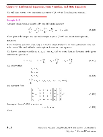
A fourth−order system is described by the differential equation

4 3 2
dy
d y
d y
d y a --------- + a -------- + a ------ + a yt() = ut() (5.106)
--------- +
dt 4 3 dt 3 2 dt 2 1 dt 0
where yt() is the output and ut() is any input. Express (5.106) as a set of state equations.
Solution:

The differential equation of (5.106) is of fourth−order; therefore, we must define four state vari-
ables that will be used with the resulting four first−order state equations.

,
,
We denote the state variables as x x x 3 , and x 4 , and we relate them to the terms of the given
1
2
differential equation as
2
3
------
---------
x = yt() x = dy x = d y x = d y (5.107)
---------
3
4
2
1
dt dt 2 dt 3
We observe that
·
x = x 2
1
·
x = x 3
2
·
x = x 4 (5.108)
3
4
d y x = – a x a x – a x a x + ut()
·
–
–
--------- =
dt 4 4 0 1 1 2 2 3 3 4
and in matrix form
x · 1 0 1 0 0 x 1 0
x · 2 = 0 0 1 0 x 2 + 0 ut() (5.109)
x · 3 0 0 0 1 x 3 0
x · 4 a – 0 a – 1 a – 2 a – 3 x 4 1
In compact form, (5.109) is written as
·
x = Ax + bu (5.110)
where

5−26 Numerical Analysis Using MATLAB® and Excel®, Third Edition

Copyright © Orchard Publications