Page 186 - Numerical Analysis Using MATLAB and Excel

Expressing Differential Equations in State Equation Form

where x · k denotes the derivative of the state variable x k .

From (5.96) through (5.99), we obtain the state equations
·
x = x 2
1
1
·
x = – R 2 -------x + 1 jωt (5.100)
---jωe
---x –
1
2
LC
L
L
It is convenient and customary to express the state equations in matrix form. Thus, we write the
state equations of (5.100) as
x · 1 = 0 1 x 1 + 0 u (5.101)
1
1
-------
--- x
x · 2 – LC – R 2 --- jωe jωt
L
L
We usually write (5.101) in a compact form as
·
x = Ax + bu (5.102)
where
·
x = x · 1 , A = 0 1 , x = x 1 , b = 1 0 jωt , and u = any input (5.103)
1
R
x · 2 – ------- – --- x 2 --- jωe
LC
L
L
The output yt() is expressed by the state equation
y = Cx + du (5.104)
where is another matrix, and is a column vector. Therefore, the state representation of a sys-
d
C
tem can be described by the pair of the of the state space equations
·
x = Ax + bu
(5.105)
y = Cx + du

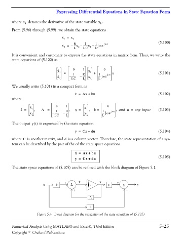
The state space equations of (5.105) can be realized with the block diagram of Figure 5.1.

+ x · x +
u b Σ ∫ dt C Σ y
+ +

A

d

Figure 5.4. Block diagram for the realization of the state equations of (5.105)

Numerical Analysis Using MATLAB® and Excel®, Third Edition 5−25

Copyright © Orchard Publications