Page 189 - Numerical Analysis Using MATLAB and Excel

Chapter 5 Differential Equations, State Variables, and State Equations

(
·
d
x t() = αe α t – t ) 0 x + αe αt ∫ t e – ατ βu τ() τ + e [ αt e – ατ βu τ() ] τ = t
0
t 0
(
α t – t ) αt t – ατ αt – αt
= α e 0 x + e ∫ e βu τ() τ + e e βut()
d
0
t 0
(
(
·
x t()= α e α t – t ) 0 x + ∫ t e α t – τ ) βu τ() τ + βut() (5.116)
d
0
t 0
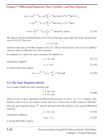
We observe that the bracketed terms of (5.116) are the same as the right side of the assumed solu-
tion of (5.113). Therefore,
·
x = αx + βu
and this is the same as the first equation of (5.111). The second equation of (5.111) is an algebraic
equation whose coefficients are scalar constants.
In summary, if and are scalar constants, the solution ofα β

·
x = αx + βu (5.117)
with initial condition
x = xt() (5.118)
0
0
is obtained from the relation
α t – t ) 0 αt t – ατ
(
xt() = e x + e ∫ e βu τ() τ (5.119)
d
0
t 0
5.9 The State Transition Matrix

Let us again consider the state equations pair
·
x = Ax + bu (5.120)
y = Cx + du

where for two or more simultaneous differential equations and are 2 × 2 or higher order
C
A
matrices, and and are column vectors with two or more rows. In this section we will intro-
b
d
duce the state transition matrix e At , and we will prove that the solution of the matrix differential
equation
·
x = Ax + bu (5.121)
with initial conditions
xt () = x 0 (5.122)
0
is obtained from the relation

5−28 Numerical Analysis Using MATLAB® and Excel®, Third Edition

Copyright © Orchard Publications