Page 194 - Numerical Analysis Using MATLAB and Excel

Computation of the State Transition Matrix

3. We obtain the coefficients from
a
i
2 n – 1 λ t
1
a + a λ + a λ + … + a n – 1 λ 1 = e
1
2
1
1
0
2
2
a + a λ + a λ + … + a n – 1 λ n – 1 = e λ t
1
0
2
2
2
2
…
2
λ
n
a + a λ + a λ + … + a n – 1 n n – 1 = e λ t
0
2 n
1 n
We use as many equations as the number of the eigenvalues, and we solve for the coefficients
a i .
4. We substitute the coefficients into the state transition matrix of (5.141), and we simplify.
a
i
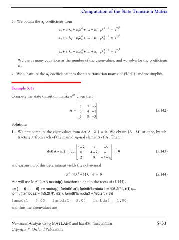
Example 5.17
Compute the state transition matrix e At given that
5 7 – 5
A = 0 4 – 1 (5.142)
2 8 – 3
Solution:

1. We first compute the eigenvalues from det A λI–[ ] = 0 . We obtain A λI–[ ] at once, by sub-
tracting from each of the main diagonal elements of . Then,
λ
A
5 – λ 7 – 5
]
[
det A λI = det 0 4 λ – 1 = 0 (5.143)
–
–
2 8 – 3 – λ
and expansion of this determinant yields the polynomial

2
3
λ – 6λ + 11λ – 6 = 0 (5.144)
We will use MATLAB roots(p) function to obtain the roots of (5.144).
p=[1 −6 11 −6]; r=roots(p); fprintf(' \n'); fprintf('lambda1 = %5.2f \t', r(1));...

fprintf('lambda2 = %5.2f \t', r(2)); fprintf('lambda3 = %5.2f', r(3))
lambda1 = 3.00 lambda2 = 2.00 lambda3 = 1.00
and thus the eigenvalues are

Numerical Analysis Using MATLAB® and Excel®, Third Edition 5−33

Copyright © Orchard Publications