Page 195 - Numerical Analysis Using MATLAB and Excel

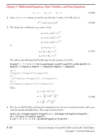
Chapter 5 Differential Equations, State Variables, and State Equations

λ = 1 λ = 2 λ = 3 (5.145)
1
2
3
2. Since is a 3 × 3 matrix, we need to use the first terms of (5.134), that is,
A
3
e At = a I + a A + a A 2 (5.146)
0
1
2
3. We obtain the coefficients a a and a, 0 1 , 2 from
2 λ t
1
a + a λ + a λ = e
0
1
2
1
1
2
2
a + a λ + a λ = e λ t
2
2
1
0
2
2
3
a + a λ + a λ = e λ t
0
3
3
2
1
or
a + a + a = e t
0
1
2
a + 2a + 4a = e 2t (5.147)
2
1
0
a + 3a + 9a = e 3t
0
1
2
We will use the following MATLAB script for the solution of (5.147).
B=sym('[1 1 1; 1 2 4; 1 3 9]'); b=sym('[exp(t); exp(2*t); exp(3*t)]'); a=B\b; fprintf(' \n');...
disp('a0 = '); disp(a(1)); disp('a1 = '); disp(a(2)); disp('a2 = '); disp(a(3))
a0 =
3*exp(t)-3*exp(2*t)+exp(3*t)
a1 =
-5/2*exp(t)+4*exp(2*t)-3/2*exp(3*t)
a2 =
1/2*exp(t)-exp(2*t)+1/2*exp(3*t)
Thus,
t
2t
a = 3e – 3e + e 3t
0
2t
--e +
a = – 5 t 4e – 3 3t (5.148)
-
--e
-
1
2
2
2t
--e
-
---e –
a = 1 t e + 1 3t
2
2
2
4. We also use MATLAB to perform the substitution into the state transition matrix, and to per-
form the matrix multiplications. The script is shown below.
syms t; a0 = 3*exp(t)+exp(3*t)−3*exp(2*t); a1 = −5/2*exp(t)−3/2*exp(3*t)+4*exp(2*t);...
a2 = 1/2*exp(t)+1/2*exp(3*t)−exp(2*t);...
A = [5 7 −5; 0 4 −1; 2 8 −3]; eAt=a0*eye(3)+a1*A+a2*A^2
5−34 Numerical Analysis Using MATLAB® and Excel®, Third Edition
Copyright © Orchard Publications