Page 200 - Numerical Analysis Using MATLAB and Excel

Eigenvectors

X ≠ 0 . This vector is called eigenvector. Obviously, there is a different eigenvector for each
X
eigenvalue. Eigenvectors are generally expressed as unit eigenvectors, that is, they are normalized to
unit length. This is done by dividing each component of the eigenvector by the square root of the
sum of the squares of their components, so that the sum of the squares of their components is
equal to unity.

⋅
In many engineering applications the unit eigenvectors are chosen such that XX T = I where
X T is the transpose of the eigenvector , and is the identity matrix.X I
Two vectors and are said to be orthogonal if their inner (dot) product is zero. A set of eigen-
X
Y
vectors constitutes an orthonormal basis if the set is normalized (expressed as unit eigenvectors)
and these vector are mutually orthogonal. An orthonormal basis can be formed with the Gram−
Schmidt Orthogonalization Procedure; it is discussed in Chapter 14.

The example which follows, illustrates the relationships between a matrix , its eigenvalues, and
A
eigenvectors.

Example 5.19

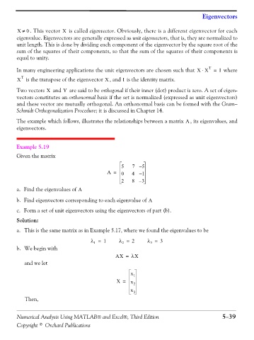
Given the matrix

5 7 – 5
A = 0 4 – 1

2 8 – 3
a. Find the eigenvalues of A

b. Find eigenvectors corresponding to each eigenvalue of A
c. Form a set of unit eigenvectors using the eigenvectors of part (b).

Solution:
a. This is the same matrix as in Example 5.17, where we found the eigenvalues to be

λ = 1 λ = 2 λ = 3
3
2
1
b. We begin with
AX = λX
and we let
x 1
X = x 2
x 3

Then,

Numerical Analysis Using MATLAB® and Excel®, Third Edition 5−39

Copyright © Orchard Publications