Page 202 - Numerical Analysis Using MATLAB and Excel

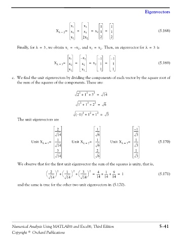
Eigenvectors

x 1 x 2 1 1
X λ = 2 = x 2 = x 2 = x 2 1 = 1 (5.168)

x 3 2x 2 2 2

Finally, for λ = 3 , we obtain x = – x 2 , and x = x 2 . Then, an eigenvector for λ = 3 is
3
1
x 1 – x 2 – 1 – 1
X λ = 3 = x 2 = x 2 = x 2 1 = 1 (5.169)
x 3 x 2 1 1

c. We find the unit eigenvectors by dividing the components of each vector by the square root of
the sum of the squares of the components. These are:

2
2
2
2 + 1 + 3 = 14
2
2
2
1 + 1 + 2 = 6
2
2
– ( 1 ) 2 + 1 + 1 = 3
The unit eigenvectors are

2 1 – 1
---------- ------- -------
14 6 3
1
1
1
Unit X λ = 1 = ---------- Unit X λ = 2 = ------- Unit X λ = 3 = ------- (5.170)
14 6 3
1
2
3
---------- ------- -------
14 6 3
We observe that for the first unit eigenvector the sum of the squares is unity, that is,
3
1
2
1
9
4
⎛ ---------- ⎞ 2 + ⎛ ---------- ⎞ 2 + ⎛ ---------- ⎞ 2 = ------ + ------ + ------ = 1 (5.171)
⎝ 14 ⎠ ⎝ 14 ⎠ ⎝ 14 ⎠ 14 14 14
and the same is true for the other two unit eigenvectors in (5.170).

Numerical Analysis Using MATLAB® and Excel®, Third Edition 5−41

Copyright © Orchard Publications