Page 193 - Numerical Analysis Using MATLAB and Excel

Chapter 5 Differential Equations, State Variables, and State Equations

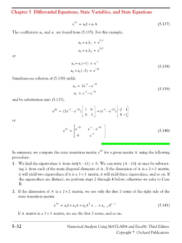
e At = a I + a A (5.137)
1
0
The coefficients and are found from (5.135). For this example,
a
a
1
0
λ t
a + a λ = e 1
0
1
1
λ t
2
a + a λ = e
0
1
2
or
(
)
a + a – 1 = e t – (5.138)
0
1
(
)
a + a – 2 = e – 2t
1
0
Simultaneous solution of (5.138) yields
t –
a = 2e – e – 2t (5.139)
0
t –
a = e – e – 2t
1
and by substitution into (5.137),
t –
t –
)
e At = ( 2e – e – 2t ) 10 + ( e – e – 2t – 2 1
–
0 1 01
or
t –
e At = e – 2t e – e – 2t (5.140)
0 e t –
In summary, we compute the state transition matrix e At for a given matrix using the following
A
procedure:
1. We find the eigenvalues from det A λI–[ ] = 0 . We can write A λI–[ ] at once by subtract-
λ
ing from each of the main diagonal elements of . If the dimension of is a 2 × 2 matrix,
λ
A
A
it will yield two eigenvalues; if it is a 3 × 3 matrix, it will yield three eigenvalues, and so on. If
the eigenvalues are distinct, we perform steps 2 through 4 below; otherwise we refer to Case
II.
2. If the dimension of is a 2 × 2 matrix, we use only the first 2 terms of the right side of the
A
state transition matrix

2
e At = a I + a A + a A + … + a n – 1 A n – 1 (5.141)
0
2
1
If matrix is a 3 × 3 matrix, we use the first 3 terms, and so on.
A
5−32 Numerical Analysis Using MATLAB® and Excel®, Third Edition

Copyright © Orchard Publications